Chapter 8 Regression and Classification Trees
## Linking to ImageMagick 6.9.12.3
## Enabled features: cairo, fontconfig, freetype, heic, lcms, pango, raw, rsvg, webp
## Disabled features: fftw, ghostscript, x11
Now we are going to turn to a very different statistical approach, called decision trees. This approach is focused on prediction of our outcome \(y\) based on covariates \(x\). Unlike our previous regression and logistic regression approaches, decision trees are a much more flexible model and are primarily focused on accurate prediction of the \(y\), but they also give a very simple and interpretable model for the data \(y\).
Decision trees, themselves, are not very powerful for predictions. However, when we combine them with ideas of resampling, we can combine together many decision trees (run on different samples of the data) to get what are called Random Forests. Random Forests are a pretty powerful and widely-used prediction tool.
8.1 Basic Idea of Decision Trees.
The basic idea behind decision trees is the following: Group the \(n\) subjects in our observed data (our training data) into a bunch of groups. The groups are defined based on binning the explanatory variables (\(x\)) of the observed data, and the bins are picked so that the observed data in a bin have similar outcomes \(y\).
Prediction for a future subject is then done in the following way. Look at the explanatory variable values for the future subject to figure into which binned values of the \(x\) the observation belongs. Then predict the future response based on the responses in the observed data that were in that group.
When the output \(y\) is continuous, we call it regression trees, and we will predict a future response based on the mean of the training data in that group/bin. If the outcome \(y\) is binary we call this technique classification trees. Just like with regression and logistic regression, there are important distinctions in how the model is built for continuous and binary data, but there is a general similarity in the approach.
8.2 The Structure of Decision Trees
The main thing to understand here is how the grouping of the data into groups is
constructed. Let’s return to the bodyfat data from our multiple regression chapter.
The groups of data are from partitioning (or binning) the \(x\) covariates in the training data. For example, one group of data in our training data could be observations that meet all of the following criterion:
HEIGHT>72.5- 91<
ABDOMEN<103 - 180<
WEIGHT<200
Notice that this group of observations is constructed by taking a simple range for each of the variables used. This is the partitioning of the \(x\) data, and decision trees limit themselves to these kind of groupings of the data. The particular values for those ranges are picked, as we said before, based on what best divides the training data so that the response \(y\) is similar.
Why Trees?
The reason these are called decision trees, is that you can describe the rules for how to put an observation into one of these groups based on a simple decision tree.
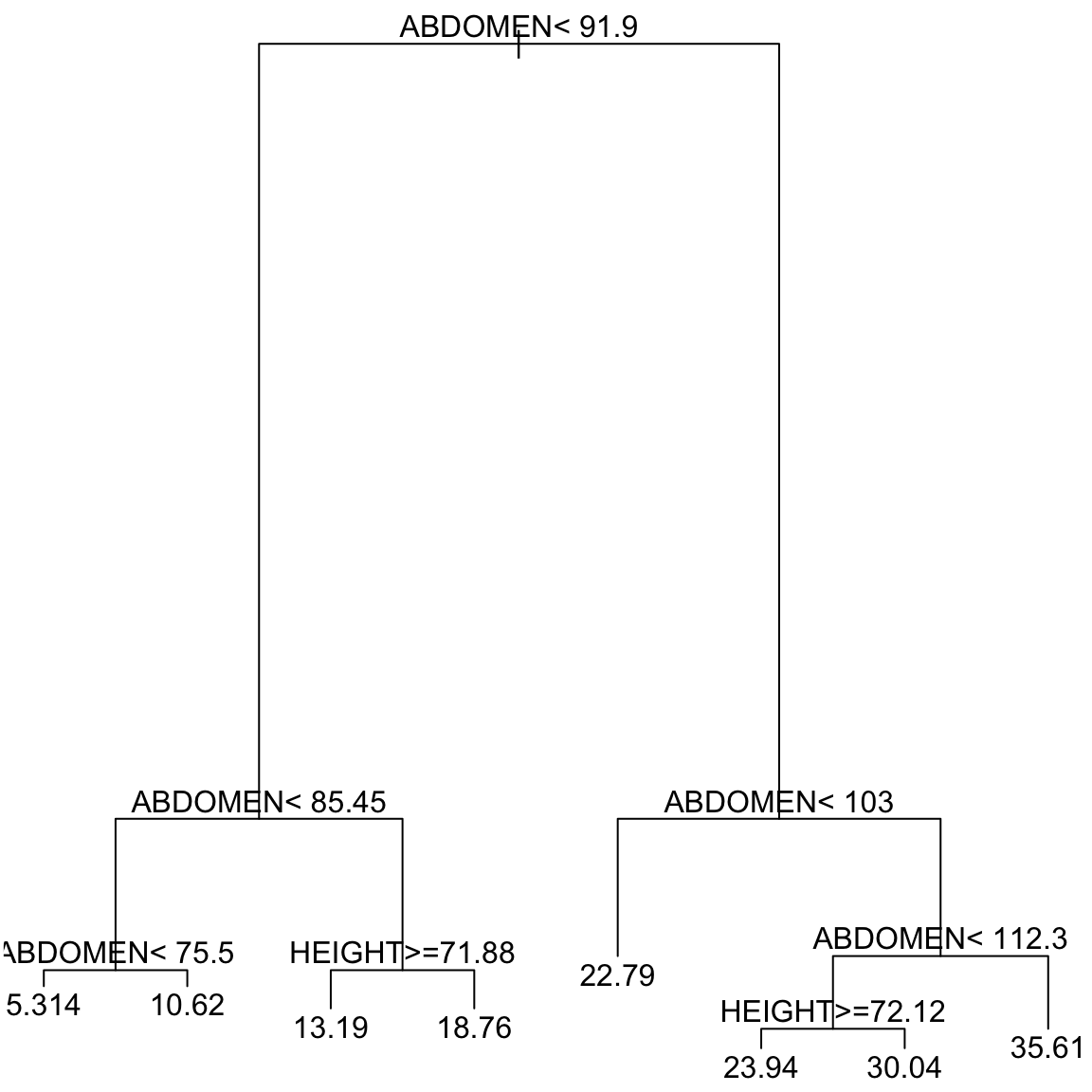
How to interpret this tree? This tree defines all of the possible groups based on the explanatory variables. You start at the top node of the tree. At each node of the tree, there is a
condition involving a variable and a cut-off. If the condition is met, then
we go left and if it is not met, we go right. The bottom “terminal nodes” or “leaves” of the tree correspond to the groups. So for example, consider an individual who is 30 years of age, 180 pounds in weight, 70 inches
tall and whose chest circumference is 95 cm, abdomen circumference is
90 cm, hip circumference is 100 cm and thigh circumference is 60
cm. The clause at the top of the tree is “ABDOMEN \(<\) 91.9” which is
met for this person, so we move left. We then encounter the clause
“ABDOMEN \(<\) 85.45” which is not met so we move right. This leads to
the clause "HEIGHT \(>=\) 71.88’’ which is true for this person. So we
move left. We then hit a terminal node, so this defines the group for this individual. Putting all those conditions together, we have that individuals in this group are defined by
- 85.45 \(\leq\)
ABDOMEN\(<\) 91.9 HEIGHT\(\geq\) 71.88
There is a displayed value for this group of \(13.19\) – this is the predicted value for individuals in this group, namely the mean of the training data that fell into this group.
Consider another terminal node, with the displayed (predicted) value of \(30.04\). What is the set of conditions that describes the observations in this group?
8.2.1 How are categorical explanatory variables dealt with?
For a categorical explanatory variable, it clearly does not make sense to put a numerical cut-off across its value. For such variables, the groups (or splits) are created by the possible combinations of the levels of the categorical variables.
Specifically, suppose \(X_j\) is a categorical variable that one of \(k\) values given by: \(\{a_1, \dots,a_k\}.\) Then possible conditions in the node of our tree are given by subsets of these \(k\) values; the condition is satisfied if the value of \(X_j\) for the observation is in this subset: go left if \(X_j \in S\) and go right if \(X_j \notin S\).
Here is an example with categorical explanatory variables from our
college dataset. The variable CONTROL corresponded to the type of college (private, public, or for profit)
Note that CONTROL is a categorical variable. Here is a decision tree based on the college data:
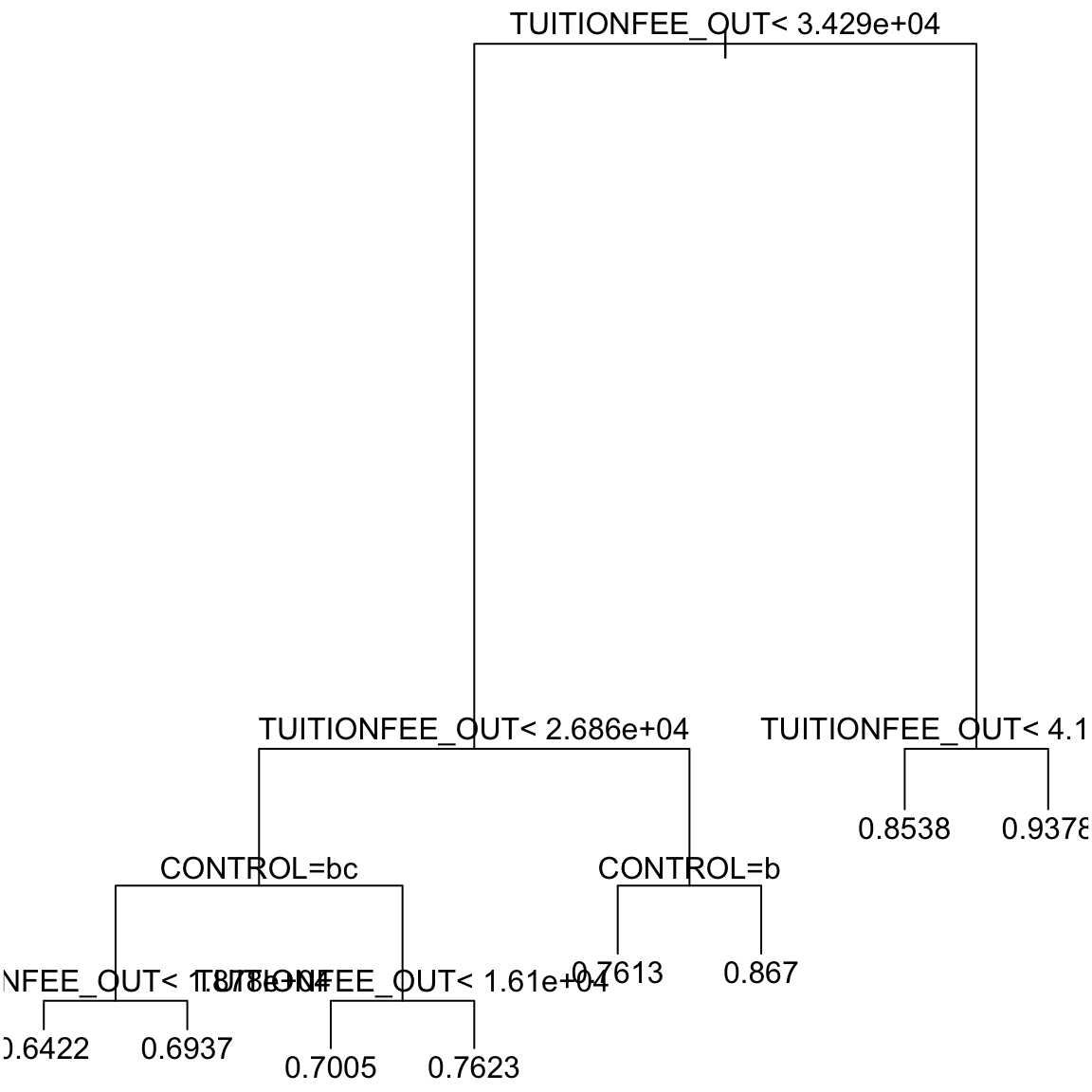 Note the conditions
 CONTROL = bc and
CONTROL = b appearing in the tree. Unfortunately the plotting command doesn’t actually give the names of the levels in the tree, but uses “a”,“b”,… for the levels. We can see the levels of CONTROL:
## [1] "public" "private" "for-profit"So in CONTROL = b, “b” corresponds to the second level of the variable, in this case “private”. So it is really CONTROL="private". CONTROL = bc corresponds CONTROL being either “b” or “c”, i.e. in either the second OR third level of CONTROL. This translates to observations where CONTROL is either “private”` OR “for-profit”. (We will also see when we look at the R command that is creating these trees below that you can work with the output to see this information better, in case you forget.)
What are the set of conditions that define the group with prediction 0.7623?
8.3 The Recursive Partitioning Algorithm
Finding the “best” such grouping or partitioning is a computationally challenging task, regardless of how we define “best”. In practice, a greedy algorithm, called Recursive Partitioning, is employed which produces a reasonable grouping, albeit not guaranteeing to be the best grouping.
8.3.1 Fitting the Tree in R
Let’s first look at how we create the above trees in R. Recursive Partitioning is done in R via the function rpart
from the library rpart.
Let us first use the rpart function to fit a regression tree
to the bodyfat dataset. We will use BODYFAT as our response, and explanatory variables Age, Weight, Height, Chest, Abdomen, Hip and
Thigh. This is, in fact, the code that gave us the tree above.
library(rpart)
rt = rpart(BODYFAT ~ AGE + WEIGHT + HEIGHT + CHEST +
    ABDOMEN + HIP + THIGH, data = body)
Notice we use a similar syntax as lm and glm to define the variable that is the response and those that are the explanatory variables.
In addition to plotting the tree, we can look at a textual representation (which can be helpful if it is difficult to see all of the tree or you want to be sure you remember whether you go right or left)
## n= 252
##
## node), split, n, deviance, yval
##       * denotes terminal node
##
##  1) root 252 17578.99000 19.150790
##    2) ABDOMEN< 91.9 132  4698.25500 13.606060
##      4) ABDOMEN< 85.45 66  1303.62400 10.054550
##        8) ABDOMEN< 75.5 7   113.54860  5.314286 *
##        9) ABDOMEN>=75.5 59  1014.12300 10.616950 *
##      5) ABDOMEN>=85.45 66  1729.68100 17.157580
##       10) HEIGHT>=71.875 19   407.33790 13.189470 *
##       11) HEIGHT< 71.875 47   902.23110 18.761700 *
##    3) ABDOMEN>=91.9 120  4358.48000 25.250000
##      6) ABDOMEN< 103 81  1752.42000 22.788890 *
##      7) ABDOMEN>=103 39  1096.45200 30.361540
##       14) ABDOMEN< 112.3 28   413.60000 28.300000
##         28) HEIGHT>=72.125 8    89.39875 23.937500 *
##         29) HEIGHT< 72.125 20   111.04950 30.045000 *
##       15) ABDOMEN>=112.3 11   260.94910 35.609090 *
Note that the tree here only uses the variables Abdomen and Height even though we gave many other variables. The other variables are not being used. This is because the algorithm, which we will discuss below, does variable selection in choosing the variables to use to split up observations.
Interaction Terms
You should note that rpart gives an error if you try to put in
interaction terms. This is because interaction is intrinsically included in decision trees
trees. You can see this by thinking about what an interaction is in our regression framework: giving a different coefficient for variable \(X_j\) based on what the value of another variable \(X_k\) is. For example, in our college data, a different slope for the variable TUITIONFEE_OUT based on whether the college is private or public is an interaction between TUITIONFEE_OUT and CONTROL.
Looking at our decision trees, we can see that the groups observations are put in also have this property – the value of TUITIONFEE_OUT that puts you into one group will also depend on the value of CONTROL. This is an indication of how much more flexible decision trees are in their predictions than linear regression.
8.3.2 How is the tree constructed?
How does rpart construct this tree? Specifically, at each node of the tree,
there is a condition involving a variable and a cut-off. How does
rpart choose the variable and the cut-off?
The first split
Let us first understand how the first condition is selected at the top of the tree, as this same process is repeated iteratively.
We’re going to assume that we have a continuous response (we’ll discuss variations to this procedure for binary response in the next section).
Our condition is going to consist of a variable and a cutoff \(c\), or if the variable is categorical, a subset \(S\) of levels. For simplicity of notation, let’s just assume that we are looking only at numerical data so we can assume for each condition we need to find a variable \(j\) and it’s corresponding cutoff \(c\), i.e. the pair \((j,c)\). Just remember for categorical variables it’s really \((j,S)\).
We are going to consider each possible variable and a possible cutoff \(c\) find the best \((j,c)\) pair for dividing the data into two groups. Specifically, each \((j,c)\) pair, can divide the subjects into two groups:
- \(G_1\) given by observations with \(X_j\leq c\)
- \(G_2\) given by observations with \(X_j > c\).
Then we need to evaluate which \((j,c)\) pair gives the best split of the data.
For any particular split, which defines groups \(G_1\) and \(G_2\), we have a predicted value for each group, \(\hat{y}_{1}\) and \(\hat{y}_2\), corresponding to the mean of the observations in group \(G_1\) and \(G_2\) (i.e. \(\bar{y}_1\) and \(\bar{y}_2\)). This means that we can calculate the loss (or error) in our prediction for each observation. Using standard squared-error loss, this gives us the RSS for the split defined by \((j,c)\): \[\begin{equation*} RSS(j, c) := \sum_{i \in G_1} (y_i - \bar{y}_1)^2 + \sum_{i \in G_2} (y_i - \bar{y}_2)^2. \end{equation*}\]
To find the best split, then, we compare the values \(RSS(j, c)\) and pick the value of \(j\) and \(c\) for which \(RSS(j, c)\) is the smallest.
Further splits
The above procedure gives the first node (or split) of the data. The same process continues down the tree, only now with a smaller portion of the data.
Specifically, the first node split the data into two groups \(G_1\) and \(G_2\). The next step of the algorithm is to repeat the same process, only now with only the data in \(G_1\) and \(G_2\) separately. Using the data in group \(G_1\) you find the variable \(X_j\) and cutoff \(c\) that divides the observations in \(G_1\) into two groups \(G_{11}\) and \(G_{12}\). You find that split by determining the pair \((j,c)\) with the smallest \(RSS\), just like before. And similarly the observations in \(G_2\) are split into two by a different pair \((j,c)\), obtaining groups \(G_{21}\) and \(G_{22}\).
This process continues, continuing to split the current sets of groups into two each time.
Measuring the improvement due to the split
Just like in regression, the improvement in fit can be quantified by comparing the error you get from adding variables (RSS) to the error you would have if you just used the group mean (TSS). This same principle applies here. For each split \((j,c)\), the smallest RSS, \[\min_{j, c} RSS(j, c)\] can be compared with the to the total variability in the data before splitting \[TSS = \sum_{i} (y_i - \bar{y})^2.\] Notice that TSS here is only calculated on the current set of observations in the group you are trying to split.
The ratio \[\frac{\min_{j, c} RSS(j, c)}{TSS}\] is always smaller than 1 and the smaller it is, the greater we are gaining by the split.
For example, for the bodyfat dataset, the total sum of squares before any splitting is 17578.99. After splitting based on ``Abdomen \(<\) 91.9’’, one gets two groups with residuals sums of squares given by 4698.255 and 4358.48. Therefore the reduction in the sum of squares is:
## [1] 0.5152022The reduction in error due to this split is therefore 0.5152. This is the greatest reduction possible by splitting the data into two groups based on a variable and a cut-off.
In the visualization of the decision tree, the length of the branches in the plot of the tree are proportional to the reduction in error due to the split. In the bodyfat dataset, the reduction in sum of squares due to the first split was 0.5152. For this dataset, this is apparently a big reduction compared to subsequence reductions and this is why it is plotted with such a long branch down to subsequent splits (a common phenomena).
For every regression tree \(T\), we can define its global RSS in the following way. Let the final groups generated by \(T\) be \(G_1, \dots, G_k\). Then the RSS of \(T\) is defined as \[\begin{equation*} RSS(T) := \sum_{j = 1}^m \sum_{i \in G_j} \left(y_i - \bar{y}_j \right)^2 \end{equation*}\] where \(\bar{y}_1, \dots, \bar{y}_m\) denote the mean values of the response in each of the groups.
We can also define a notion of \(R^2\) for the regression tree as: \[\begin{equation*} R^2(T) := 1 - \frac{RSS(T)}{TSS}. \end{equation*}\]
## [1] 0.73541958.3.3 Tree Size and Pruning
Notice that as we continue to recursively split our groups, we have less and less data each time on which to decide how to split the data. In principle we could keep going until each group consisted of a single observation! Clearly we don’t want to do that, which brings us to the biggest and most complicated issue for decision trees. How large should the tree be “grown”? Very large trees obviously lead to over-fitting, but insufficient number of splits will lead to poor prediction. We’ve already seen a similar over-fitting phenomena in regression, where the more variables you include the better the fit will be on your training data. Decision trees are have a similar phenomena only it is based on how big the tree is – bigger trees will fit the training data better but may not generalize to new data well creating over-fitting.
How is rpart deciding when to
stop growing the tree?
In regression we saw that we could make this choice via cross-validation – we fit our model on a portion of the tree and then evaluated it on the left out portion. This is more difficult to conceptualize for trees. Specifically, with regression, we could look at different a priori submodels (i.e. subset of variables), fit the submodels to our random subsets of data, and calculate the cross-validation error for each submodel to choose the best one. For our decision trees, however, what would be our submodels be? We could consider different variables as input, but this wouldn’t control the size of the tree, which is a big source of over-fitting.
One strategy is to instead stop when the improvement
\[\frac{\min_{(j,c)}RSS(j, c )}{TSS}\]
is not very large. This would be the case when we are not
gaining all that much by splitting further. This is actually not a
very smart strategy. Why? Because you can actually sometimes split the data and get small amount of improvements, but because you were able to split the data there, it allows you to make another split later that adds a lot of improvement. Stopping the first time you see a small improvement would keep you from discovering that future improvement.
Regression and classification trees were invented by Leo Breiman from UC Berkeley. He also had a different approach for the tree size issue. He advocated against stopping the recursive partitioning algorithm. Instead, he recommends growing a full tree (or a very large tree), \(T_{\max}\), and then “pruning” back \(T_{\max}\) by cutting back lower level groupings. This allows you to avoid situations like above, where you miss a great split because of an early unpromising split. This “pruned” tree will be a subtree of the full tree.
How to Prune
The idea behind pruning a tree is to find a measure of how well a smaller (prunned) tree is fitting the data that doesn’t suffer from the issue that larger trees will always fit the training data better. If you think back to variable selection in regression, in addition to cross-validation, we also have measures in addition to cross-validation, like CP, AIC, and BIC, that didn’t involve resampling, but had a form \[R(\alpha)=RSS + \alpha k\] In other words, use RSS as a measure of fit, but penalize models with a large number of variables \(k\) by adding a term \(\alpha k\). Minimizing this quantity meant that smaller models with good fits could have a value \(R(\alpha)\) that was lower than bigger models.
Breiman proposed a similar strategy for measuring the fit of a potential subtree for pruning, but instead penalizing for the size of the tree rather than the number of variables. Namely, for a possible subtree \(T\), define \[\begin{equation*} R_{\alpha}(T) := RSS(T) + \alpha (TSS) |T| \end{equation*}\] where \(|T|\) is the number of terminal nodes of the tree \(T\). \(R_{\alpha}(T)\) is evaluated for all the possible subtrees, and the subtree with the smallest \(R_{\alpha}(T)\) is chosen. Since it depends on \(\alpha\), we will call the subtree that minimizes \(R_{\alpha}(T)\) \(T(\alpha)\).
Obviously the number of possible subtrees and possible values of \(\alpha\) can be large, but there is an algorithm (weakest link cutting) that simplifies the process. In fact it can be shown that only a fixed number of \(\alpha_k\) values and the corresponding optimal \(T(\alpha_k)\) subtrees need to be considered. In other words you don’t need to consider all \(\alpha\) values, but only a fixed set of \(\alpha_k\) values and compare the fit of their optimal \(T(\alpha_k)\) subtree.
After obtaining this sequence
of trees \(T(\alpha_1), T(\alpha_2), \dots\), the default choice in R is
to take \(\alpha* = 0.01\) and then generating the tree \(T(\alpha_k)\) for the \(\alpha_k\) closest to \(\alpha*\).68 The value of \(\alpha^*\) is set by the argument cp in rpart.
The \(printcp()\) function in R gives those fixed \(\alpha_k\) values for this data and also gives the number of splits of the subtrees \(T(\alpha_k)\) for each \(k\):
##
## Regression tree:
## rpart(formula = BODYFAT ~ AGE + WEIGHT + HEIGHT + CHEST + ABDOMEN +
##     HIP + THIGH, data = body)
##
## Variables actually used in tree construction:
## [1] ABDOMEN HEIGHT
##
## Root node error: 17579/252 = 69.758
##
## n= 252
##
##         CP nsplit rel error  xerror     xstd
## 1 0.484798      0   1.00000 1.01231 0.082170
## 2 0.094713      1   0.51520 0.62743 0.054181
## 3 0.085876      2   0.42049 0.53554 0.048519
## 4 0.024000      3   0.33461 0.40688 0.036850
## 5 0.023899      4   0.31061 0.41292 0.036841
## 6 0.012125      5   0.28672 0.37323 0.031539
## 7 0.010009      6   0.27459 0.37330 0.029112
## 8 0.010000      7   0.26458 0.38678 0.029401
Each row in the printcp output corresponds to a different tree \(T(\alpha_k)\). Note that each tree has an increasing number of splits. This is a property of the \(T(\alpha_k)\) values, specifically that the best trees for each \(\alpha_k\) value will be nested within each other, so going from \(\alpha_k\) to \(\alpha_{k+1}\) corresponds to adding an additional split to one of the terminal nodes of \(T(\alpha_k)\).
Also given in the printcp output are three other quantities:
rel error: for a tree \(T\) this simply \(RSS(T)/TSS\). Because more deep trees have smaller RSS, this quantity will always decrease as we go down the column.xerror: an accuracy measure calculated by 10-fold cross validation (and then divided by TSS). Notice before we mentioned the difficult in conceptualizing cross-validation. But now that we have the complexity parameter \(\alpha\), we can use this for cross-validation. Instead of changing the number of variables \(k\) and comparing the cross-validated error, we can change values of \(\alpha\), fit the corresponding tree on random subsets of the data, and evaluate the cross-validated error as to which value of \(\alpha\) is better. Notice that this quantity will be random (i.e., different runs of \(rpart()\) will result in different values forxerror); this is because 10-fold cross-validation relies on randomly partitioning the data into 10 parts and the randomness of this partition results inxerrorbeing random.xstd: The quantityxstdprovides a standard deviation for the random quantityxerror. If we do not like the default choice of 0.01 for \(\alpha\), we can choose a higher value of \(\alpha\) using \(xerror\) and \(xstd\).
For this particular run, the xerror seems to be smallest at \(\alpha = 0.012125\) and then xerror seems to increase. So we could give this value to the argument
cp in rpart instead of the default cp = 0.01.
rtd = rpart(BODYFAT ~ AGE + WEIGHT + HEIGHT + CHEST +
ABDOMEN + HIP + THIGH, data = body, cp = 0.0122)
plot(rtd)
text(rtd)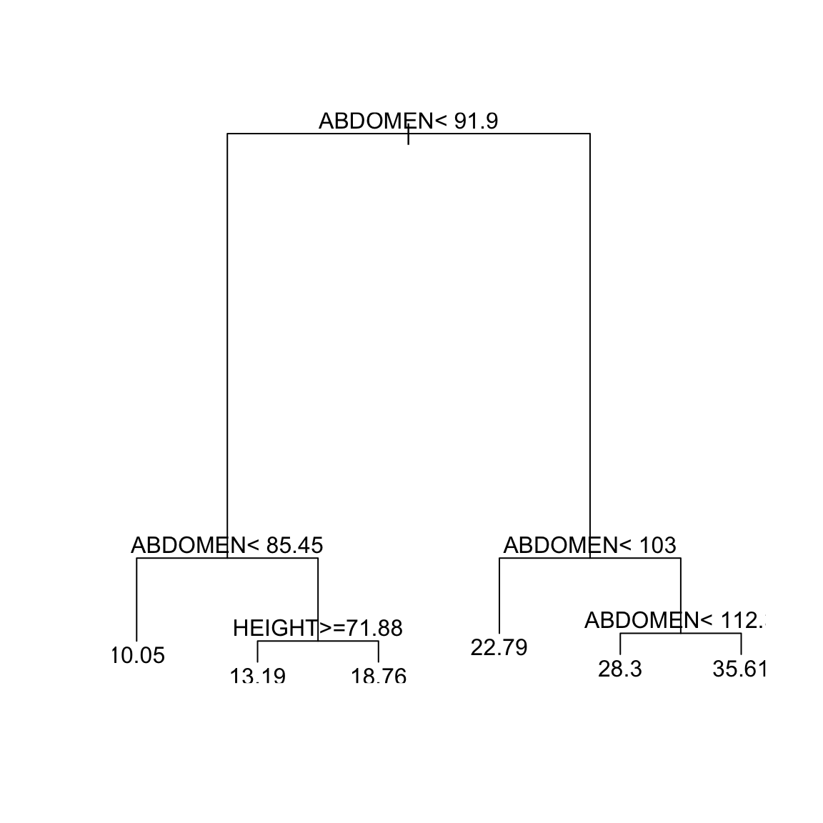 We will then get a smaller
tree. Now we get a tree with 5 splits or 6 terminal nodes.
We will then get a smaller
tree. Now we get a tree with 5 splits or 6 terminal nodes.
However, we would also note that xstd is around \(0.032=0.033\), so it’s not clear that the difference between the xerror values for the different \(\alpha\) values is terribly meaningful.
8.3.4 Classification Trees
The partitioning algorithm for classification trees (i.e. for a 0-1 response) is the same, but we need to make sure we have an appropriate measurement for deciding on which split is best at each iteration, and there are several to choose from. We can still use the \(RSS\) for binary response, which is the default in R, in which case it has a useful simplification that we will discuss.
Specifically, as in the case of regression trees, we need to find the pair \((j,c)\) corresponding to a variable \(X_j\) and a cut-off \(c\). (or a pair \((j,S)\) for variables \(X_j\) that are categorical). Like regression trees, the pair \((j,c)\) divides the observations into the two groups \(G_1\) (where \(X_j \leq c\)) and \(G_2\) (where \(X_j > c\)), and we need to find the pair \((j,c)\) that gives the best fit to the data. We will go through several measures.
8.3.4.1 RSS / Gini-Index
We can use the RSS as before,
\[\begin{equation*}
RSS(j, c) := \sum_{i \in G_1} (y_i - \bar{y}_1)^2 + \sum_{i \in G_2}
(y_i - \bar{y}_2)^2
\end{equation*}\]
where \(\bar{y}_1\) and \(\bar{y}_2\) denote the mean values of the
response in the groups \(G_1\) and \(G_2\) respectively. Since in classification
problems the response values are 0 or 1, \(\bar{y}_1\) equals
the proportion of ones in \(G_1\) while \(\bar{y}_2\) equals the
proportion of ones in \(G_2\). It is therefore better to denote \(\bar{y}_1\) and
\(\bar{y}_2\) by \(\hat{p}_1\) and \(\hat{p}_2\) respectively,
so that the formula for \(RSS(j, c)\) then simplifies to:
\[\begin{equation*}
RSS(j, c) = n_1 \hat{p}_1 (1 - \hat{p}_1) + n_2 \hat{p}_2 (1 -
\hat{p}_2).
\end{equation*}\]
This quantity is also called the Gini index of the split
corresponding to the pair \((j,c)\).
Notice that the Gini index involves calculating the function
\(p(1-p)\) for each group’s proportion of \(1\)’s:
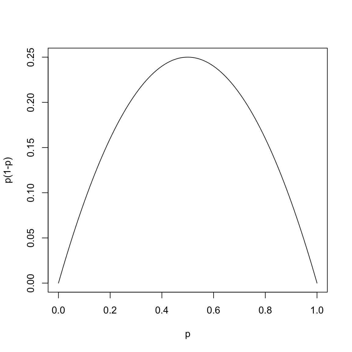
This function takes its largest value at \(p = 1/2\) and it is small when \(p\) is close to 0 or 1.
Therefore the quantity \[n_1 \hat{p}_1 (1 - \hat{p}_1)\] is small if either most of the response values in the group \(G_1\) are 0 (in which case \(\hat{p}_1\) is close to \(0\)) or when most of the response values in the group are 1 (in which case \(\hat{p}_1 \approx 1\)).
A group is said to be pure if either most of the response values in the group are 0 or if most of the response values are 1. Thus the quantity \(n_1 \hat{p}_1 (1 - \hat{p}_1)\) measures the impurity of a group. If \(n_1 \hat{p}_1 (1 - \hat{p}_1)\) is low, then the group is pure and if it is high, it is impure. The group is maximally impure if \(\hat{p}_1 = 1/2\).
The Gini Index (which is \(RSS(j, c)\)), is the sum of the impurities of the groups defined by the split given by \(X_j \leq c\) and \(X_j > c\). So that for binary data, the recursive partitioning algorithm determines \(j\) and \(c\) as the one that divides the observations into two groups with high amount of purity.
8.3.4.2 Other measures
The quantity \(n \hat{p} (1 - \hat{p})\) is not the only function used for measuring the impurity of a group in classification. The key property of the function \(p(1 - p)\) is that it is symmetric about \(1/2\), takes its maximum value at \(1/2\) and it is small near the end points \(p = 0\) and \(p = 1\). Two other functions having this property are also commonly used:
- Cross-entropy or Deviance: Defined as \[-2n \left(\hat{p} \log \hat{p} + (1 - \hat{p}) \log (1 - \hat{p}) \right).\] This also takes its smallest value when \(\hat{p}\) is 0 or 1 and it takes its maximum value when \(\hat{p} = 1/2\). We saw this value when we did logistic regression, as a measure of the fit.
Misclassification Error: This is defined as \[n \min(\hat{p}, 1 - \hat{p}).\] This quantity equals 0 when \(\hat{p}\) is 0 or 1 and takes its maximum value when \(\hat{p} = 1/2\).
This is value is called misclassification error based on prediction using a majority rule decision for prediction. Specifically, assume we predict the response for an observation in group \(G\) based on the which response is seen the most in group \(G\). Then the number of observations that are misclassified by this rule will be equal to \(n \min(\hat{p}, 1 - \hat{p}).\)
One can use Deviance or Misclassification error instead of the Gini index while growing a classification tree. The default in R is to use the Gini index.
8.3.4.3 Application to spam email data
Let us apply the classification tree to the email spam dataset from the chapter on logistic regression.
The only change to the rpart function to classification is to use the argument
method = "class".
sprt = rpart(yesno ~ crl.tot + dollar + bang + money +
    n000 + make, method = "class", data = spam)
plot(sprt)
text(sprt)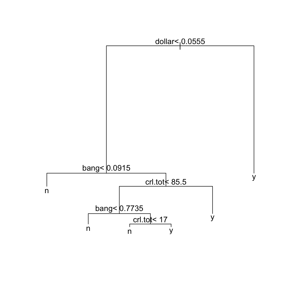
The tree construction works exactly as in the regression tree. We can
look at the various values of the \(\alpha_k\) parameter and the
associated trees and errors using the function printcp.
##
## Classification tree:
## rpart(formula = yesno ~ crl.tot + dollar + bang + money + n000 +
##     make, data = spam, method = "class")
##
## Variables actually used in tree construction:
## [1] bang    crl.tot dollar
##
## Root node error: 1813/4601 = 0.39404
##
## n= 4601
##
##         CP nsplit rel error  xerror     xstd
## 1 0.476558      0   1.00000 1.00000 0.018282
## 2 0.075565      1   0.52344 0.54661 0.015380
## 3 0.011583      3   0.37231 0.38445 0.013414
## 4 0.010480      4   0.36073 0.38886 0.013477
## 5 0.010000      5   0.35025 0.38886 0.013477
Notice that the xerror seems to decrease as cp decreases. We might
want to set the cp to be lower than 0.01 so see how the xerror
changes:
sprt = rpart(yesno ~ crl.tot + dollar + bang + money +
    n000 + make, method = "class", cp = 0.001, data = spam)
printcp(sprt)
##
## Classification tree:
## rpart(formula = yesno ~ crl.tot + dollar + bang + money + n000 +
## make, data = spam, method = "class", cp = 0.001)
##
## Variables actually used in tree construction:
## [1] bang crl.tot dollar money n000
##
## Root node error: 1813/4601 = 0.39404
##
## n= 4601
##
## CP nsplit rel error xerror xstd
## 1 0.4765582 0 1.00000 1.00000 0.018282
## 2 0.0755654 1 0.52344 0.55764 0.015492
## 3 0.0115830 3 0.37231 0.38886 0.013477
## 4 0.0104799 4 0.36073 0.37397 0.013262
## 5 0.0063431 5 0.35025 0.37341 0.013254
## 6 0.0055157 10 0.31660 0.35190 0.012930
## 7 0.0044126 11 0.31109 0.34859 0.012879
## 8 0.0038610 12 0.30667 0.33094 0.012599
## 9 0.0027579 16 0.29123 0.32984 0.012581
## 10 0.0022063 17 0.28847 0.33315 0.012635
## 11 0.0019305 18 0.28627 0.33260 0.012626
## 12 0.0016547 20 0.28240 0.33205 0.012617
## 13 0.0010000 25 0.27413 0.32874 0.012563Now the minimum xerror seems to be the tree with 16 splits (at cp = 0.0027). A reasonable choice of cp here is therefore \(0.0028\). We
can refit the classification tree with this value of cp:
sprt = rpart(yesno ~ crl.tot + dollar + bang + money +
    n000 + make, method = "class", cp = 0.0028, data = spam)
plot(sprt)
text(sprt)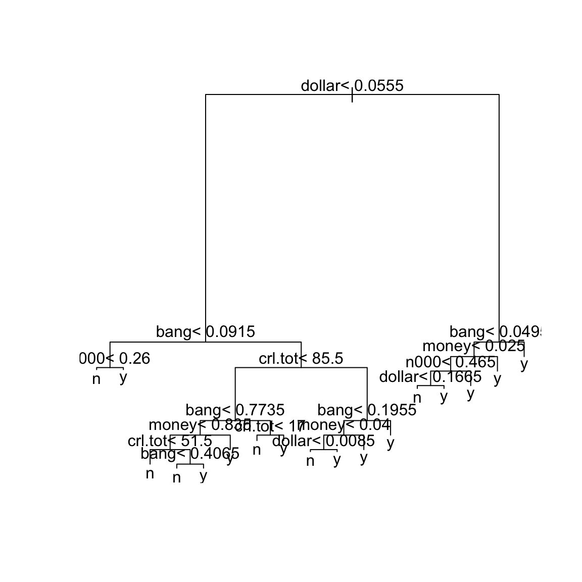
Predictions for Binary Data
Let us now talk about getting predictions from the classification
tree. Prediction is obtained in the usual way using the predict
function. The predict function results in predicted probabilities
(not 0-1 values). Suppose we have an email where crl.tot = 100,
dollar = 3, bang = 0.33, money = 1.2, n000 = 0 and make = 0.3. Then the predicted probability for this email being spam is
given by:
x0 = data.frame(crl.tot = 100, dollar = 3, bang = 0.33,
    money = 1.2, n000 = 0, make = 0.3)
predict(sprt, newdata = x0)
## n y
## 1 0.04916201 0.950838The predicted probability is 0.950838. If we want to convert this into a 0-1 prediction, we can do this via a confusion matrix in the same way as for logistic regression.
y = as.numeric(spam$yesno == "y")
y.hat = predict(sprt, spam)[, 2]
v <- seq(0.1, 0.9, by = 0.05)
tree.conf = confusion(y, y.hat, thres = v)
plot(v, tree.conf[, "W1"] + tree.conf[, "W0"], xlab = "threshold",
    ylab = "Total error", type = "l")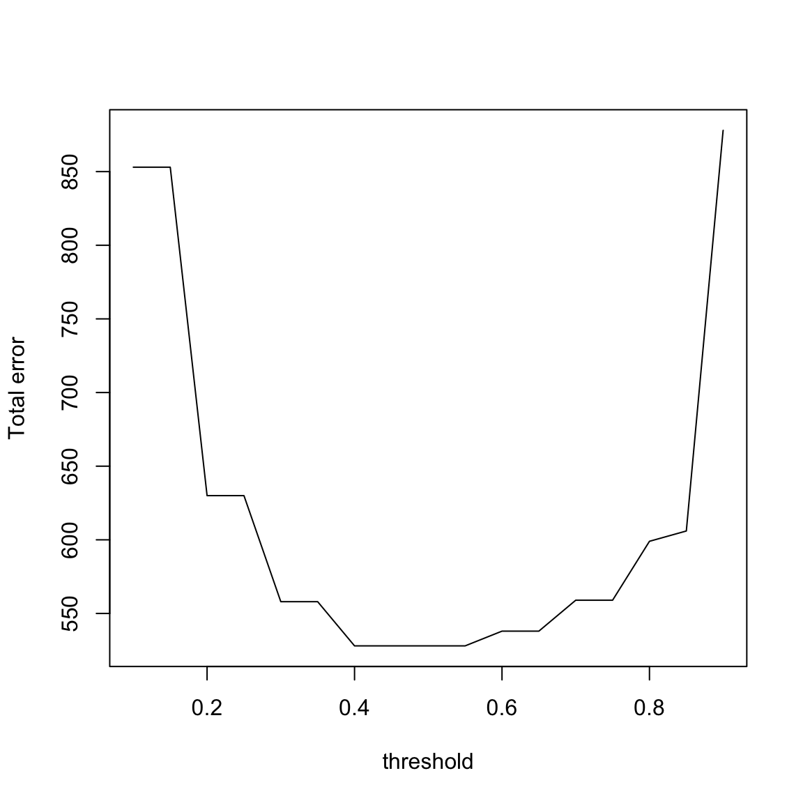
It seems that it is pretty equivalent between \(0.4-0.6\), so it is seems the simple choice of 0.5 is reasonable. This would give the following confusion matrix:
| \(\hat{y} = 0\) | \(\hat{y} = 1\) | |
| \(y = 0\) | \(C_0=2624\) | \(W_1=164\) |
| \(y = 1\) | \(W_0=364\) | \(C_1=1449\) |
8.4 Random Forests
Decision trees are very simple and intuitive, but they often do not perform well in prediction compare to other techniques. They are too variable, with the choice of variable \(X_j\) and the cutoff \(c\) changing a good deal with small changes in the data. However, decisions trees form the building blocks for a much better technique called random forests. Essentially a random forest is a collection of decision trees (either regression or classification trees depending on the type of response).
The idea behind random forests is to sample from your training data (like in the bootstrap) to create new datasets, and fit decision trees to each of these resampled data. This gives a large number of decision trees, from similar but not exactly the same data. Then the prediction of a new observation is based on combining the predictions of all these trees.69
8.4.1 Details of Constructing the Random Trees
We will construct \(B\) total trees. The method for constructing the \(b^{th}\) tree (for \(b = 1, \dots, B\)) is the following:
- Generate a new dataset having \(n\) observations by resampling uniformly at random with replacement from the existing set of observations. This resampling is the same as in bootstrap. Of course, some of the original set of observations will be repeated in this bootstrap sample (because of with replacement draws) while some other observations might be dropped altogether. The observations that do not appear in the bootstrap are referred to as out of bag (o.o.b) observations.
- Construct a decision tree based on
the bootstrap sample. This tree construction is almost the same as
the construction underlying the
rpartfunction but with two important differences:
Random selection of variables At each stage of splitting the data into groups, \(k\) number of variables are selected at random from the available set of \(p\) variables and only splits based on these \(k\) variables are considered. In contrast, in
rpart, the best split is chosen by considering possible splits from all \(p\) explanatory variables and all thresholds.So it can happen, for example, that the first split in the tree is chosen from variables \(1, 2, 3\) resulting in two groups \(G_1\) and \(G_2\). But then in splitting the group \(G_1\), the split might chosen from variables \(4, 5, 6\) and in further splitting group \(G_2\), the next split might be based on variables \(1, 5, 6\) and so on.
The rationale behind this random selection of variables is that often covariates are highly correlated with each other, and the choice of using one \(X_j\) versus a variable \(X_k\) is likely to be due to training observations you have. Indeed we’ve seen in the body fat data, that the variables are highly correlated with each other. On future data, a different variable \(X_k\) might perform better. So by actually forcing the tree to explore not always relying on \(X_j\), you are more likely to give good predictions for future data that may not match your training data.
No “pruning” of trees We discussed above how to choose the depth or size of a tree, noting that too large of a tree results in a tree with a lot of variability, as your groups are based on small sample sizes. However, the tree construction in random forests the trees are actually grown to full size. There is no pruning involved, i.e. no attempt to find the right size tree. More precisely, each tree is grown till the number of observations in each terminal node is no more than a size \(m\). This, of course, means that each individual tree will overfit the data. However, each individual tree will overfit in a different way and when we average the predictions from different trees, the overfitting will be removed.
At the end, we will have \(B\) trees. These \(B\) trees will all be different because each tree will be based on a different bootstrapped dataset and also because of our randomness choice of variables to consider in each split. The idea is that these different models, that might be roughly similar, when put together will fit future data more robustly.
Prediction now works in the following natural way. Given a new observation with explanatory variable values \(x_1, \dots, x_p\), each tree in our forest will yield a prediction for the response of this new observation. Our final prediction will simply take the average of the predictions of the individual trees (in case of regression trees) or the majority vote of the predictions of the individual trees in case of classification.
8.4.2 Application in R
We shall use the R function randomForest (in the package
randomForest) for constructing random forests. The following important parameters are
ntreecorresponding to \(B\), the number of trees to fit. This should be large (default choice is 500)mtrycorresponding to \(k\), the number of random variables to consider at each split (whose default choice is \(p/3\))nodesizecorresponding to \(m\), the maximum size allowed for any terminal node (whose default size is 5)
Let us now see how random forests work for regression in the bodyfat dataset.
The syntax for the randomForest function works as follows:
library(randomForest)
ft = randomForest(BODYFAT ~ AGE + WEIGHT + HEIGHT +
    CHEST + ABDOMEN + HIP + THIGH, data = body, importance = TRUE)
ft
##
## Call:
## randomForest(formula = BODYFAT ~ AGE + WEIGHT + HEIGHT + CHEST + ABDOMEN + HIP + THIGH, data = body, importance = TRUE)
## Type of random forest: regression
## Number of trees: 500
## No. of variables tried at each split: 2
##
## Mean of squared residuals: 23.30256
## % Var explained: 66.6R tells us that ntree is 500 and mtry (number of variables tried
at each split) is 2. We can change these values if we want.
The square of the mean of squared residuals roughly indicates the size of each residual. These residuals are slightly different from the usual residuals in that for each observation, the fitted value is computed from those trees where this observation is out of bag. But you can ignore this detail.
The percent of variance explained is similar to
\(R^2\). The importance = TRUE clause inside the randomForest function
gives some variable importance measures. These can be seen by:
##          %IncMSE IncNodePurity
## AGE      9.84290      1003.557
## WEIGHT  13.47958      2206.806
## HEIGHT  13.27250      1200.290
## CHEST   15.54825      3332.758
## ABDOMEN 36.10359      5729.390
## HIP     12.79099      2013.501
## THIGH   12.01310      1424.241
The exact meaning of these importance measures is nicely described in the help entry for the function importance. Basically, large values indicate these variables were important for the prediction, roughly because many of the trees built as part of the random forest used these variables.
The variable ABDOMEN seems to be the
most important (this is unsurprising given our previous experience
with this dataset) for predicting bodyfat.
Now let us come to prediction with random forests. The R command for
this is exactly the same as before. Suppose we want to the body fat
percentage for a new individual whose AGE = 40, WEIGHT = 170, HEIGHT = 76, CHEST = 120, ABDOMEN = 100, HIP = 101 and THIGH = 60. The
prediction given by random forest for this individual’s response is
obtained via the function predict
x0 = data.frame(AGE = 40, WEIGHT = 170, HEIGHT = 76,
    CHEST = 120, ABDOMEN = 100, HIP = 101, THIGH = 60)
predict(ft, x0)
## 1
## 24.12099Now let us come to classification and consider the email spam dataset. The syntax is almost the same as regression.
sprf = randomForest(as.factor(yesno) ~ crl.tot + dollar +
    bang + money + n000 + make, data = spam)
sprf
##
## Call:
## randomForest(formula = as.factor(yesno) ~ crl.tot + dollar + bang + money + n000 + make, data = spam)
## Type of random forest: classification
## Number of trees: 500
## No. of variables tried at each split: 2
##
## OOB estimate of error rate: 11.61%
## Confusion matrix:
## n y class.error
## n 2646 142 0.05093257
## y 392 1421 0.21621622The output is similar to the regression forest except that now we are also given a confusion matrix as well as some estimate of the misclassification error rate.
Prediction is obtained in exactly the same was as regression forest via:
x0 = data.frame(crl.tot = 100, dollar = 3, bang = 0.33,
    money = 1.2, n000 = 0, make = 0.3)
predict(sprf, x0)
## 1
## y
## Levels: n yNote that unlike logistic regression and classification tree, this directly gives a binary prediction (instead of a probability). So we don’t even need to worry about thresholds.