Chapter 3 Comparing Groups and Hypothesis Testing
We’ve mainly discussed informally comparing the distribution of data in different groups. Now we want to explore tools about how to use statistics to make this more formal. Specifically, how can we quantify whether the differences we see are due to natural variability or something deeper? We will do this through hypothesis testing.
In addition to reviewing specific hypothesis tests, we have the following goals:
- Abstract the ideas of hypothesis testing: in particular what it means to be “valid” and what makes a good procedure
- Dig a little deeper as to what assumptions we are making in using a particular test
- Learn about two paradigms for hypothesis testing:
- parametric methods
- resampling methods
- parametric methods
Depending on whether you took STAT 20 or Data 8, you may be more familiar with one of these paradigms than the other.
We will first consider the setting of comparing two groups, and then expand out to comparing multiple groups.
3.1 Choosing a Statistic
Example of Comparing Groups
Recall the airline data, with different airline carriers. We could ask the question about whether the distribution of flight delays is different between carriers.
If we wanted to ask whether United was more likely to have delayed flights than American Airlines, how might we quantify this?
The following code subsets to just United (UA) and American Airlines (AA) and takes the mean of DepDelay (the delay in departures per flight)
## [1] NAWhat do you notice happens in the above code when I take the mean of all our observations?
Instead we need to be careful to use na.rm=TRUE if we want to ignore NA values (which may not be wise if you recall from Chapter 2, NA refers to cancelled flights!)
## [1] 11.13185We can use a useful function tapply that will do calculations by groups. We demonstrate this function below where the variable Carrier (the airline) is a factor variable that defines the groups we want to divide the data into before taking the mean (or some other function of the data):
## AA UA
## NA NA
Again, we have a problem of NA values, but we can pass argument na.rm=TRUE to mean:
##        AA        UA
##  7.728294 12.255649
We can also write our own functions. Here I calculate the percentage of flights delayed or cancelled:
tapply(flightSubset$DepDelay, flightSubset$Carrier,
    function(x) {
        sum(x > 0 | is.na(x))/length(x)
    })
## AA UA
## 0.3201220 0.4383791These are statistics that we can calculate from the data. A statistic is any function of the input data sample.
3.2 Hypothesis Testing
Once we’ve decided on a statistic, we want to ask whether this is a meaningful difference between our groups. Specifically, with different data samples, the statistic would change. Inference is the process of using statistical tools to evaluate whether the statistic observed indicates some kind of actual difference, or whether we could see such a value due to random chance even if there was no difference.
Therefore, to use the tools of statistics – to say something about the generating process – we must be able to define a random process that we imagine created the data.
Hypothesis testing encapsulate these inferential ideas. Recall the main components of hypothesis testing:
- Hypothesis testing sets up a null hypothesis which describes a feature of the population data that we want to test – for example, are the medians of the two populations the same?
In order to assess this question, we need to know what would be the distribution of our sample statistic if that null hypothesis is true. To do that, we have to go further than our null hypothesis and further describe the random process that could have created our data if the null hypothesis is true.
If we know this process, it will define the specific probability distribution of our statistic if the null hypothesis was true. This is called the null distribution.
There are a lot of ways “chance” could have created non-meaningful differences between our populations. The null distribution makes specific and quantitative what was previously the qualitative question “this difference might be just due to chance.”
How do we determine whether the null hypothesis is a plausible explanation for the data? We take the value of the statistic we actually observed in our data, and we determine whether this observed value is too unlikely under the null distribution to be plausible.
Specifically, we calculate the probability (under the null distribution) of randomly getting a statistic \(X\) under the null hypothesis as extreme as or more extreme than the statistic we observed in our data \((x_{obs})\). This probability is called a p-value.
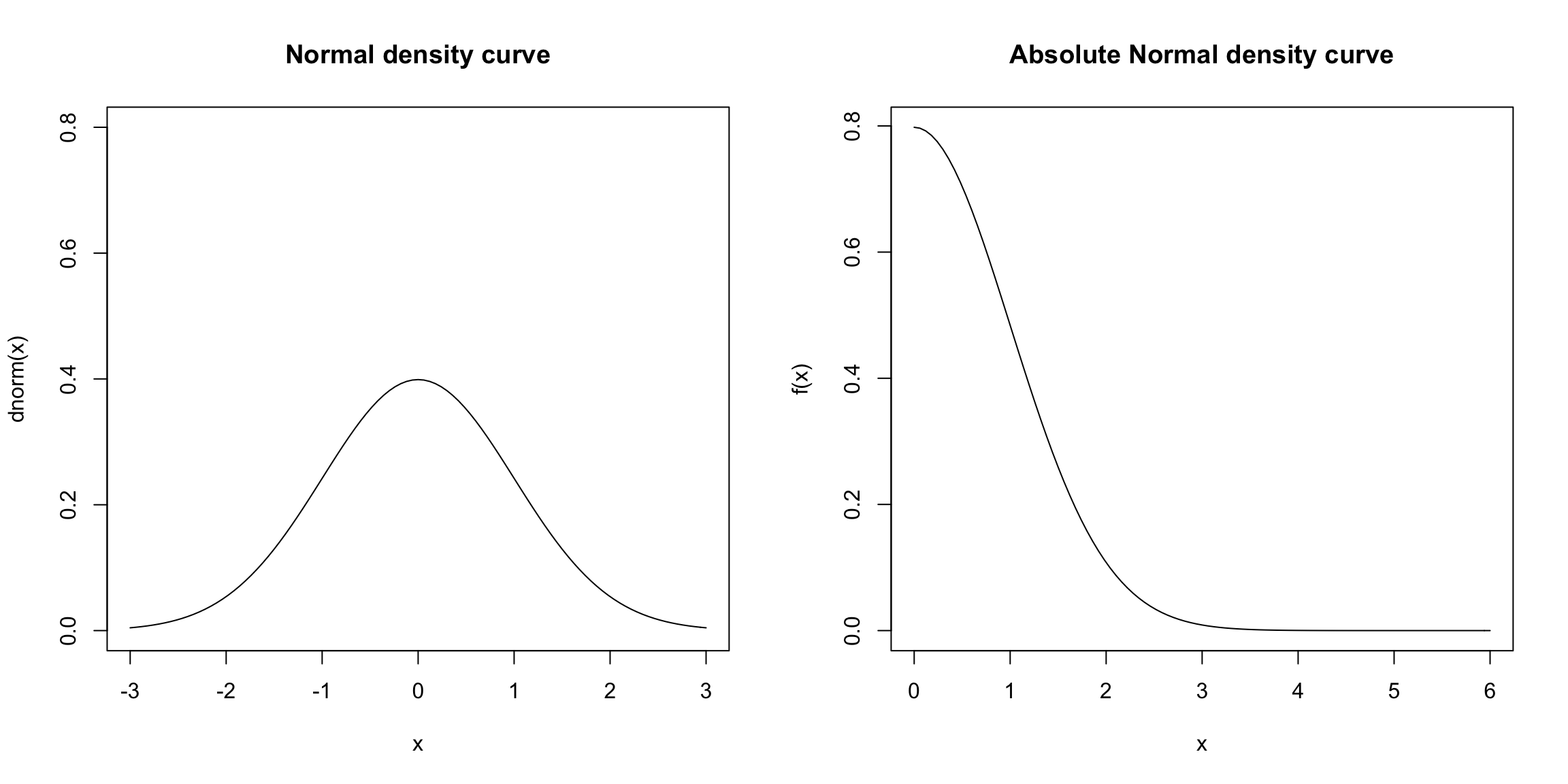
“Extreme” means values of the test-statistic that are unlikely under the null hypothesis we are testing. In almost all tests it means large numeric values of the test-statistic, but whether we mean large positive values, large negative values, or both depends on how we define the test-statistic and which values constitute divergence from the null hypothesis. For example, if our test statistic is the absolute difference in the medians of two groups, then large positive values are stronger evidence of not following the null distribution: \[\text{p-value}(x_{obs})=P_{H_0}(X \geq x_{obs})\]
If we were looking at just the difference, large positive or negative values are evidence against the null that they are the same,17 \[\text{p-value}(x_{obs})=P_{H_0}( X \leq -x_{obs}, X \geq x_{obs} )=1-P_{H_0}(-x_{obs}\leq X \leq x_{obs}).\]
Does the p-value give you the probability that the null is true?
If the observed statistic is too unlikely under the null hypothesis we can say we reject the null hypothesis or that we have a statistically significant difference.
How unlikely is too unlikely? Often a proscribed cutoff value of 0.05 is used so that p-values less than that amount are considered too extreme. But there is nothing magical about 0.05, it’s just a common standard if you have to make a “Reject”/“Don’t reject” decision. Such a standard cutoff value for a decision is called a level. Even if you need to make a Yes/No type of decision, you should report the p-value as well because it gives information about how discordant with the null hypothesis the data is.
3.2.1 Where did the data come from? Valid tests & Assumptions
Just because a p-value is reported, doesn’t mean that it is correct. You must have a valid test. A valid test simply means that the p-value (or level) that you report is accurate. This is only true if the null distribution of the test statistic is correctly identified. To use the tools of statistics, we must assume some kind of random process created the data. When your data violates the assumptions of the data generating process, your p-value can be quite wrong.
What does this mean to violate the assumptions? After all, the whole point of hypothesis testing is that we’re trying to detect when the statistic doesn’t follow the null hypothesis distribution, so obviously we will frequently run across examples where the assumption of the null hypothesis is violated. Does this mean p-values are not valid unless the null-hypothesis is true? Obviously not, other. Usually, our null hypothesis is about one specific feature of the random process – that is our actual null hypothesis we want to test. The random process that we further assume in order to get a precise null statistic, however, will have further assumptions. These are the assumptions we refer to in trying to evaluate whether it is legitimate to rely on hypothesis testing/p-values.
Sometimes we can know these assumptions are true, but often not; knowing where your data came from and how it is collected is critical for assessing these questions. So we need to always think deeply about where the data come from, how they were collected, etc.
Example: Data that is a Complete Census For example, for the airline data, we have one dataset that gives complete information about the month of January. We can ask questions about flights in January, and get the answer by calculating the relevant statistics. For example, if we want to know whether the average flight is more delayed on United than American, we calculate the means of both groups and simply compare them. End of story. There’s no randomness or uncertainty, and we don’t need the inference tools from above. It doesn’t make sense to have a p-value here.
Types of Samples
For most of statistical applications, it is not the case that we have a complete census. We have a sample of the entire population, and want to make statements about the entire population, which we don’t see. Notice that having a sample does not necessarily mean a random sample. For example, we have all of January which is a complete census of January, but is also a sample from the entire year, and there is no randomness involved in how we selected the data from the larger population.
Some datasets might be a sample of the population with no easy way to describe the process of how the sample was chosen from the population, for example data from volunteers or other convenience samples that use readily available data rather than randomly sampling from the population. Having convenience samples can make it quite fraught to try to make any conclusions about the population from the sample; generally we have to make assumptions about the data was collected, but because we did not control how the data is collected, we have no idea if the assumptions are true.
What problems do you have in trying to use the flight data on January to estimate something about the entire year? What would be a better way to get flight data?
We discussed this issue of how the data was collected for estimating histograms. There, our histogram is a good estimate of the population when our data is a i.i.d sample or SRS, and otherwise may be off base. For example, here is the difference in our density estimates from Chapter 2 applied to three different kinds of sampling, the whole month of January, a i.i.d sample from the year, and a Stratified Sample, that picked a SRS of the same size from each month of the year:
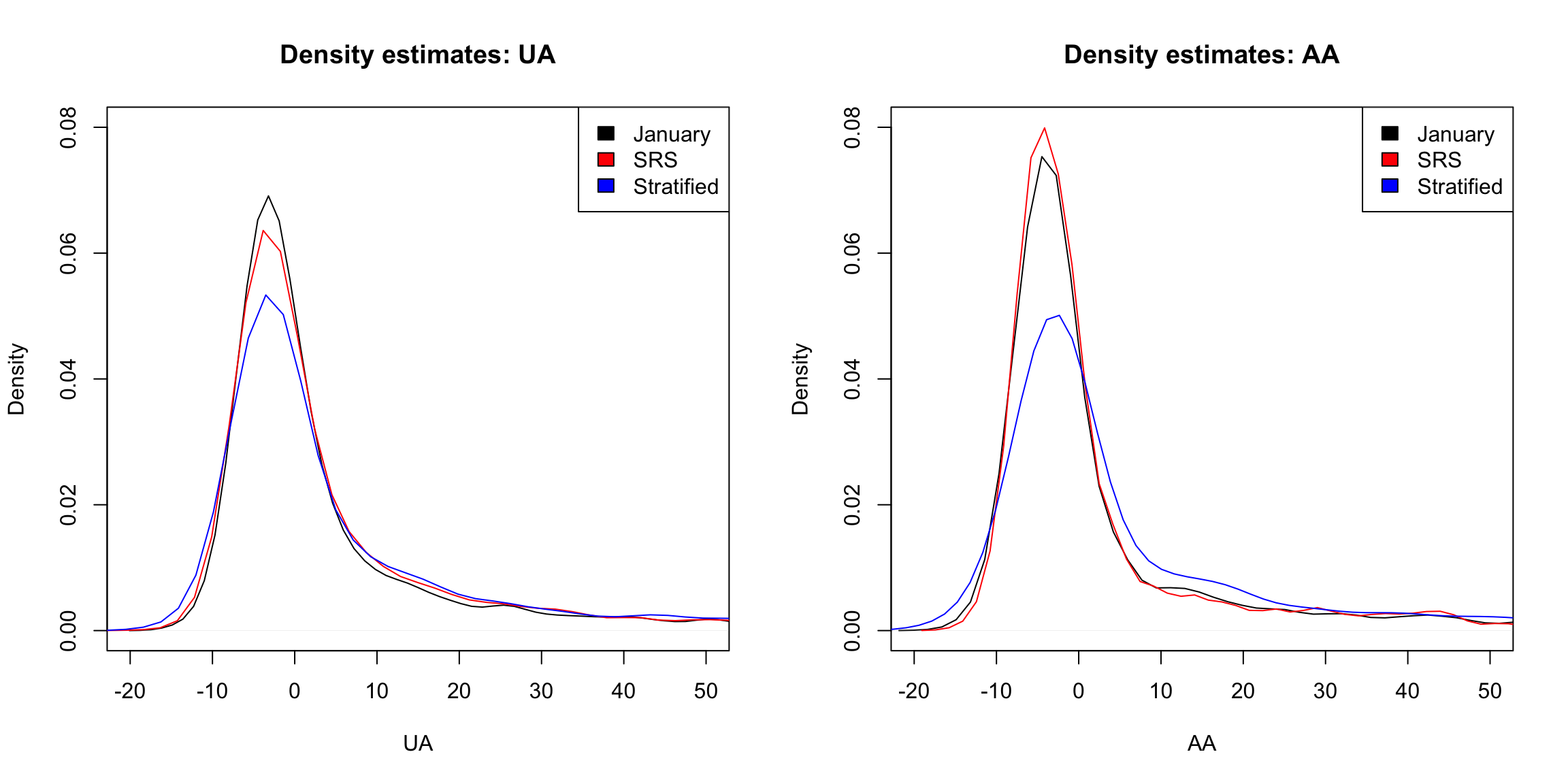
Recall in Chapter 2, that we said while the method we learned is appropriate for a SRS, there are also good estimates for other kind of random samples, like the Stratified Sample, though learning about beyond the reach of this course. The key ingredient that is needed to have trustworthy estimates is to precisely know the probability mechanism that drew the samples. This is the key difference between a random sample (of any kind), where we control the random process, and a sample of convenience – which may be random, but we don’t know how the random sample was generated.
Assumptions versus reality
A prominent statistician, George Box, gave the following famous quote,
All models are wrong but some are useful
All tests have assumptions, and most are often not met in practice. This is a continual problem in interpreting the results of statistical methods. Therefore there is a great deal of interest in understanding how badly the tests perform if the assumptions are violated; this is often called being robust to violations. We will try to emphasize both what the assumptions are, and how bad it is to have violations to the assumptions.
For example, in practice, much of data that is available is not a carefully controlled random sample of the population, and therefore a sample of convenience in some sense (there’s a reason we call them convenient!). Our goal is not to make say that analysis of such data is impossible, but make clear about why this might make you want to be cautious about over-interpreting the results.
3.3 Permutation Tests
Suppose we want to compare the the proportion of flights with greater than 15 minutes delay time of United and American airlines. Then our test statistic will be the difference between that proportion
The permutation test is a very simple, straightforward mechanism for comparing two groups that makes very few assumptions about the distribution of the underlying data. The permutation test basicallly assumes that the data we saw we could have seen anyway even if we changed the group assignments (i.e. United or American). Therefore, any difference we might see between the groups is due to the luck of the assignment of those labels.
The null distribution for the test statistic (difference of the proportion) under the null hypothesis for a permutation tests is determined by making the following assumptions:
- There is no difference between proportion of delays greater than 15 minutes between the two airlines, \[H_0:p_{UA}=p_{AA}\] This is the main feature of the null distribution to be tested
- The statistic observed is the result of randomly assigning the labels amongst the observed data. This is the additional assumption about the random process that allows for calculating a precise null distribution of the statistic. It basically expands our null hypothesis to say that the distribution of the data between the two groups is the same, and the labels are just random assignments to data that comes from the same distribution.
3.3.1 How do we implement it?
This is just words. We need to actually be able to compute probabilities under a specific distribution. In other words, if we were to have actually just randomly assigned labels to the data, we need to know what is the probablility we saw the difference we actually saw?
The key assumption is that the data we measured (the flight delay) was fixed for each observation and completely independent from the airline the observation was assigned to. We imagine that the airline assignment was completely random and separate from the flight delays – a bunch of blank airplanes on the runway that we at the last minute assign to an airline, with crew and passengers (not realistic, but a thought experiment!)
If our data actually was from such a scenario, we could actually rerun the random assignment process. How? By randomly reassigning the labels. Since (under the null) we assume that the data we measured had nothing to do with those labels, we could have instead observed another assignment of those airline labels and we would have seen the same data with just different labels on the planes. These are called permutations of the labels of the data.
Here is some examples of doing that. Below, are the results of three different possible permutations, created by assigning planes (rows/observations) to an airline randomly – only the first five observations are shown, but all of the original observations get an assignment. Notice the number of planes assigned to UA vs AA stays the same, just which plane gets assigned to which airline changes. The column Observed shows the assignment we actually saw (as opposed to the assignments I made up by permuting the assignments)
##   FlightDelay Observed Permutation1 Permutation2 Permutation3
## 1           5       UA           AA           UA           AA
## 2          -6       UA           UA           UA           UA
## 3         -10       AA           UA           UA           UA
## 4          -3       UA           UA           AA           UA
## 5          -3       UA           UA           AA           UA
## 6           0       UA           UA           UA           UA
For each of these three permutations, I can calculate proportion of flights delayed, among those assigned to UA vs those assigned to AA, and calculate the difference between them
## Proportions per Carrier, each permutation:## Observed Permutation1 Permutation2 Permutation3
## AA 0.1554878 0.2063008 0.1951220 0.1910569
## UA 0.2046216 0.1878768 0.1915606 0.1929002## Differences in Proportions per Carrier, each permutation:## Observed Permutation1 Permutation2 Permutation3
## 0.049133762 -0.018424055 -0.003561335 0.001843290I’ve done this for three permutations, but we could enumerate (i.e. list) all possible such assignments of planes to airlines. If we did this, we would have the complete set potential flight delay datasets possible under the null hypothesis, and for each one we could calculate the difference in the proportion of delayed flights between the airlines.
So in principle, it’s straightforward – I just do this for every possible permutation, and get the difference of proportions. The result set of differences gives the distribution of possible values under the null. These values would define our null distribution. With all of these values in hand, I could calculate probabilities – like the probability of seeing a value so large as the one observed in the data (p-value!).
Too many! In practice: Random selection
This is the principle of the permutation test, but I’m not about to do that in practice, because it’s not computationally feasible!
Consider if we had only, say, 14 observations with two groups of 7 each, how many permutations do we have? This is 14 “choose” 7, which gives 3,432 permutations.
So for even such a small dataset of 14 observations, we’d have to enumerate almost 3500 permutations. In the airline data, we have 984-2986 observations per airline. We can’t even determine how many permutations that is, much less actually enumerate them all.
So for a reasonably sized dataset, what can we do? Instead, we consider that there exists such a null distribution and while we can’t calculate it perfectly, we are going to just approximate that null distribution.
How? Well, this is a problem we’ve actually seen. If we want to estimate a true distribution of values, we don’t usually have a census at our disposal – i.e. all values. Instead we draw a i.i.d. sample from the population, and with that sample we can estimate that distribution, either by a histogram or by calculating probabilities (see Chapter 2).
How does this look like here? We know how to create a single random permutation – it’s what I did above using the function sample. If we repeat this over and over and create a lot of random permutations, we are creating a i.i.d. sample from our population. Specifically, each possible permutation is an element of our sample space, and we are randomly drawing a permutation. We’ll do this many times (i.e. many calls to the function sample), and this will create a i.i.d. sample of permutations. Once we have a i.i.d. sample of permutations, we can calculate the test statistic for each permutation, and get an estimate of the true null distribution. Unlike i.i.d. samples of an actual population data, we can make the size of our sample as large as our computer can handle to improve our estimate (though we don’t in practice need it to be obscenely large)
Practically, this means we will repeating what we did above many times. The function replicate in R allows you to repeat something many times, so we will use this to repeat the sampling and the calculation of the difference in medians.
I wrote a little function permutation.test to do this for any statistic, not just difference of the medians; this way I can reuse this function repeatedly in this chapter. You will go through this function in lab and also in the accompanying code.
permutation.test <- function(group1, group2, FUN, n.repetitions) {
    stat.obs <- FUN(group1, group2)
    makePermutedStats <- function() {
        sampled <- sample(1:length(c(group1, group2)),
            size = length(group1), replace = FALSE)
        return(FUN(c(group1, group2)[sampled], c(group1,
            group2)[-sampled]))
    }
    stat.permute <- replicate(n.repetitions, makePermutedStats())
    p.value <- sum(stat.permute >= stat.obs)/n.repetitions
    return(list(p.value = p.value, observedStat = stat.obs,
        permutedStats = stat.permute))
}
Example: Proportion Later than 15 minutes
We will demonstrate this procedure on our the i.i.d. sample from our flight data, using the difference in the proportions later than 15 minutes as our statistic.
Recall, the summary statistics on our actual data:
##        AA        UA
## 0.1554878 0.2046216
I am going to choose as my statistic the absolute difference between the proportion later than 15 minutes. This will mean that large values are always considered extreme for my p-value computations. This is implemented in my diffProportion function:
diffProportion <- function(x1, x2) {
    prop1 <- propFun(x1)
    prop2 <- propFun(x2)
    return(abs(prop1 - prop2))
}
diffProportion(subset(flightSFOSRS, Carrier == "AA")$DepDelay,
    subset(flightSFOSRS, Carrier == "UA")$DepDelay)
## [1] 0.04913376Now I’m going to run my permutation function using this function.
Here is the histogram of the values of the statistics under all of my permutations.
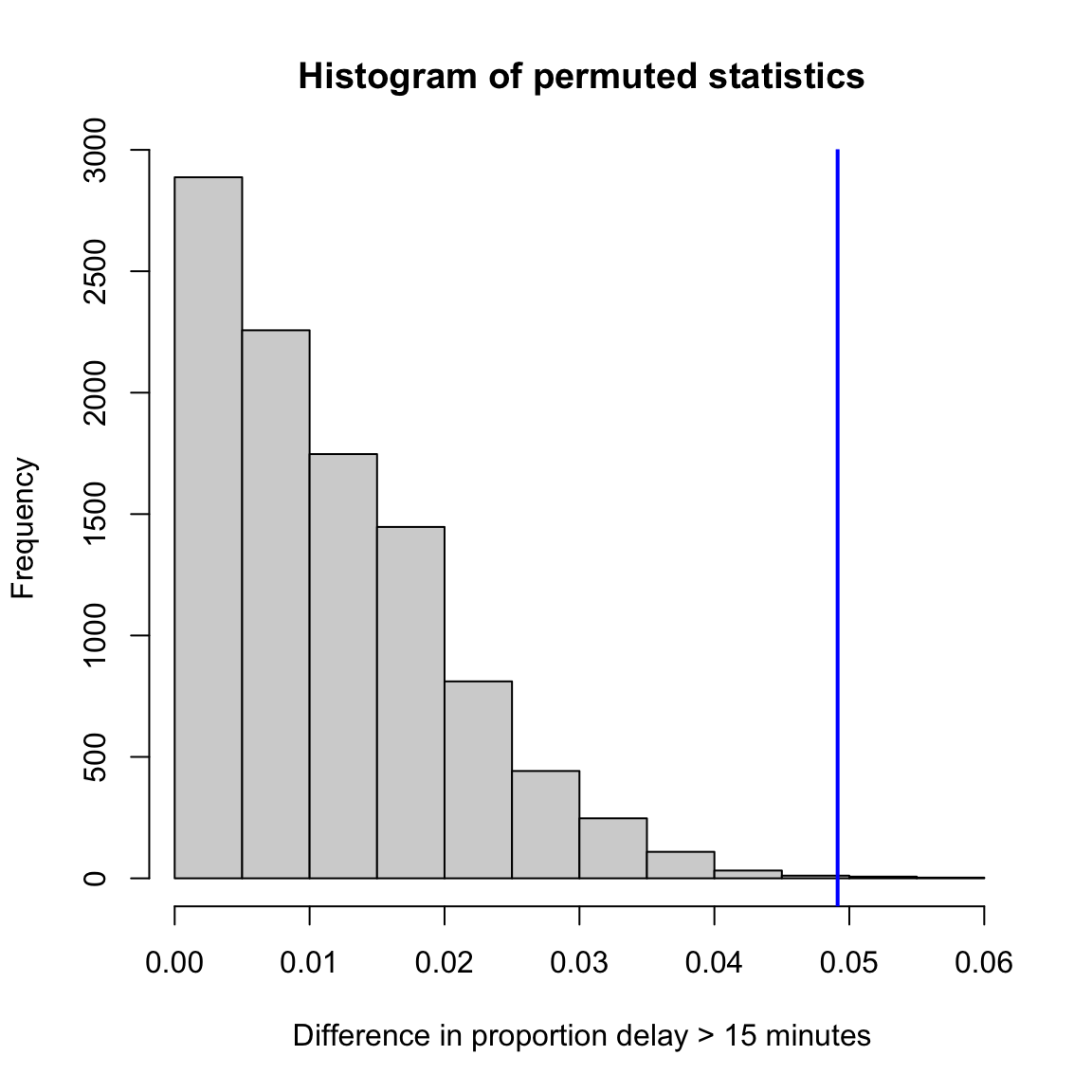
If my data came from the null, then this is the (estimate) of the actual distribution of what the test-statistic would be.
How would I get a p-value from this? Recall the definition of a p-value – the probability under the null distribution of getting a value of my statistic as large or larger than what I observed in my data, \[\text{p-value}(x_{obs})=P_{H_0}(X \geq x_{obs})\] So I need to calculate that value from my estimate of the null distribution (demonstrated in the histogram above), i.e. the proportion of the that are greater than observed.
My function calculated the p-value as well in this way, so we can output the value:
## pvalue= 0.0011- So what conclusions would you draw from this permutation test?
- What impact does this test have? What conclusions would you be likely to make going forward?
- Why do I take the absolute difference? What difference does it make if you change the code to be only the difference?
Median difference
What about if I look at the difference in median flight delay between the two airlines? Let’s first look at what is the median flight delay for each airline:
tapply(flightSFOSRS$DepDelay, flightSFOSRS$Carrier,
    function(x) {
        median(x, na.rm = TRUE)
    })[c("AA", "UA")]
## AA UA
## -2 -1The first thing we might note is that there is a very small difference between the two airlines (1 minute). So even if we find something significant, who really cares? That is not going to change any opinions about which airline I fly. Statistical significance is not everything.
However, I can still run a permutation test (you can always run tests, even if it’s not sensible!). I can reuse my previous function, but just quickly change the statistic I consider – now use the absolute difference in the median instead of proportion more than 15min late.
Here is the histogram I get after doing this:
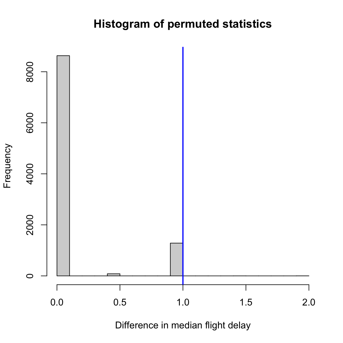 This gives us a p-value:
## pvalue (median difference)= 0.1287- What is going on with our histogram? Why does it look so different from our usual histograms?
- What would have happened if we had defined our p-value as the probability of being greater rather than greater than or equal to? Where in the code of
permutation.testwas this done, and what happens if you change the code for this example?
3.3.2 Assumptions: permutation tests
Let’s discuss what might be limitations of the permutation test.
Assumption: the data generating process
What assumption(s) are we making about the random process that generated this data in determining the null distribution? Does it make sense for our data?
We set up a model that the assignment of a flight to one airline or another was done at random. This is clearly not a plausible description of our of data.
Some datasets do have this flavor. For example, if we wanted to decide which of two email solicitations for a political campaign are most likely to lead to someone to donate money, we could randomly assign a sample of people on our mailing list to get one of the two. This would perfectly match the data generation assumed in the null hypothesis.
What if our assumption about random labels is wrong?
Clearly random assignment of labels is not a good description for how the datasets regarding flight delay data were created. Does this mean the permutation test will be invalid? No, not necessarily. In fact, there are other descriptions of null random process that do not explicitly follow this description, but in the end result in the same null distribution as that of the randomly assigned labels model.
Explicitly describing the full set of random processes that satisfy this requirement is beyond the level of this class18, but an important example is if each of your data observations can be considered under the null a random, independent draw from the same distribution. This is often abbreviated i.i.d: independent and identically distributed. This makes sense as an requirement – the very act of permuting your data implies such an assumption about your data: that you have similar observations and the only thing different about them is which group they were assigned to (which under the null doesn’t matter).
Assuming your data is i.i.d is a common assumption that is thrown around, but is actually rather strong. For example, non-random samples do not have this property, because there is no randomness; it is unlikely you can show that convenience samples do either. However, permutation tests are a pretty good tool even in this setting, however, compared to the alternatives. Actual random assignments of the labels is the strongest such design of how to collect data.
Inferring beyond the sample population
Note that the randomness queried by our null hypothesis is all about the specific observations we have. For example, in our political email example we described above, the randomness is if we imagine that we assigned these same people different email solicitations – our null hypothesis asks what variation in our statistic would we expect? However, if we want to extend this to the general population, we have to make the assumption that these people’s reaction are representative of the greater population.
As a counter-example, suppose our sample of participants was only women, and we randomly assigned these women to two groups for the two email solicitations. Then this data matches the assumptions of the permutation test, and the permutation test is valid for answering the question about whether any affect seen amongst these women was due to the chance assignment to these women. But that wouldn’t answer our question very well about the general population of interest, which for example might include men. Men might have very different reactions to the same email. This is a rather obvious example, in the sense that most people in designing a study wouldn’t make this kind of mistake. But it’s exemplifies the kind of problems that can come from a haphazard selection of participants, even if you do random assignment of the two options. Permutation tests do not get around the problem of a poor data sample. Random samples from the population are needed to be able to make the connection back to the general population.
Conclusion
So while permuting your data seems to intuitive and is often thought to make no assumptions, it does have assumptions about where your data come from.
Generally, the assumptions for a permutation test are much less than some alternative tests (like the parametric tests we’ll describe next), so they are generally the safest to use. But it’s useful to realize the limitations even for something as non-restrictive as permutation tests.
3.4 Parametric test: the T-test
In parametric testing, we assume the data comes from a specific family of distributions that share a functional form for their density, and define the features of interest for the null hypothesis based on this distribution.
Rather than resampling from the data, we will use the fact that we can write down the density of the data-generating distribution to analytically determine the null distribution of the test statistic. For that reason, parametric tests tend to be limited to a narrower class of statistics, since the statistics have to be tractable for mathematical analysis.
3.4.1 Parameters
We have spoken about parameters in the context of parameters that define a family of distributions all with the same mathematical form for the density. An example is the normal distribution which has two parameters, the mean (\(\mu\)) and the variance (\(\sigma^2\)). Knowing those two values defines the entire distribution of a normal. The parameters of a distribution are often used to define a null hypothesis; a null hypothesis will often be a direct statement about the parameters that define the distribution of the data. For example, if we believe our data is normally distributed in both of our groups, our null hypothesis could be that the mean parameter in one group is equal to that of another group.
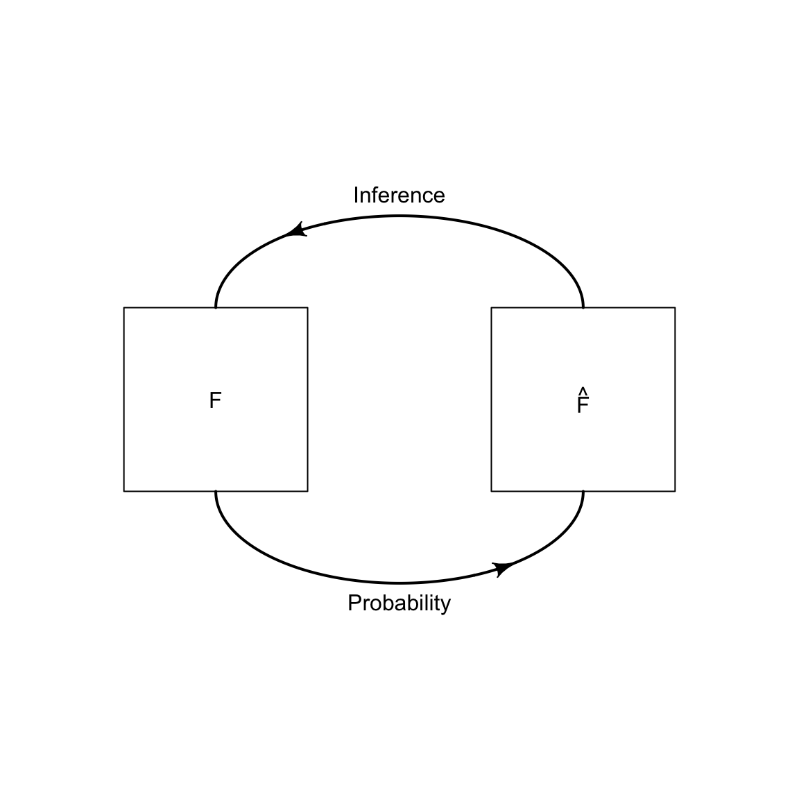
General Parameters However, we can also talk more generally about a parameter of any distribution beyond the defining parameters of the distribution. A parameter is any numerical summary that we can calculate from a distribution. For example, we could define the .75 quantile as a parameter of the data distribution. Just as a statistic is any function of our observed data, a parameter is a function of the true generating distribution \(F\). Which means that our null hypothesis could also be in terms of other parameters than just the ones that define the distribution. For example, we could assume that the data comes from a normal distribution and our null hypothesis could be about the .75 quantile of the distribution. Indeed, we don’t have to have assume that the data comes from any parametric distribution – every distribution has a .75 quantile.
If we do assume our data is generated from a family of distributions defined by specific parameters (e.g. a normal distribution with unknown mean and variance) then those parameters completely define the distribution. Therefore any arbitrary parameter of the distribution we might define can be written as a function of those parameters. So the 0.75 quantile of a normal distribution is a parameter, but it is also a function of the mean parameter and variance parameter of the normal distribution.
Notation Parameters are often indicated with greek letters, like \(\theta\), \(\alpha\), \(\beta\), \(\sigma\).
Statistics of our data sample are often chosen because they are estimates of our parameter. In that case they are often called the same greek letters as the parameter, only with a “hat” on top of them, e.g. \(\hat{\theta}\), \(\hat{\alpha}\), \(\hat{\beta}\), \(\hat{\sigma}\). Sometimes, however, a statistic will just be given a upper-case letter, like \(T\) or \(X\), particularly when they are not estimating a parameter of the distribution.
3.4.2 More about the normal distribution and two group comparisons
Means and the normal distribution play a central role in many parametric tests, so lets review a few more facts.
Standardized Values
If \(X\sim N(\mu,\sigma^2)\), then \[\frac{X-\mu}{\sigma} \sim N(0,1)\] This transformation of a random variable is called standardizing \(X\), i.e. putting it on the standard \(N(0,1)\) scale.
Sums of normals
If \(X\sim N(\mu_1,\sigma_1^2)\) and \(Y\sim N(\mu_2, \sigma_2^2)\) and \(X\) and \(Y\) are independent, then \[X+Y \sim N(\mu_1+\mu_2, \sigma_1^2+\sigma_2^2)\]
If \(X\) and \(Y\) are both normal, but not independent, then their sum is still a normal distribution with mean equal to \(\mu_1+\mu_2\) but the variance is different.19
CLT for differences of means
We’ve reviewed that a sample mean of a i.i.d. sample or SRS sample will have a sampling distribution that is roughly a normal distribution if we have a large enough sample size – the Central Limit Theorem. Namely, that if \(X_1,\ldots,X_n\) are i.i.d from a distribution20 with mean \(\mu\) and variance \(\sigma^2\), then \(\hat{\mu}=\bar{X}=\frac{1}{n}\sum_{i=1}^n X_i\) will have a roughly normal distribution \[N(\mu,\frac{\sigma^2}{n}).\]
If we have two groups,
- \(X_1,\ldots,X_{n_1}\) i.i.d from a distribution with mean \(\mu_1\) and variance \(\sigma^2_1\), and
- \(Y_1,\ldots,Y_{n_2}\) i.i.d from a distribution with mean \(\mu_2\) and variance \(\sigma^2_2\)
Then if the \(X_i\) and \(Y_i\) are independent, then the central limit theorem applies and \(\bar{X}-\bar{Y}\) will have a roughly normal distribution equal to \[N(\mu_1-\mu_2, \frac{\sigma_1^2}{n_1}+\frac{\sigma_2^2}{n_2})\]
3.4.3 Testing of means
Let \(\mu_{UA}\) and \(\mu_{AA}\) be the true means of the distribution of flight times of the two airlines in the population. Then if we want to test if the distributions have the same mean, we can write our null hypothesis as \[H_0: \mu_{AA}=\mu_{UA}\] This could also be written as \[H_0: \mu_{AA}-\mu_{UA}=\delta=0,\] so in fact, we are testing whether a specific parameter \(\delta\) is equal to \(0\).
Let’s assume \(X_1,\ldots,X_{n_1}\) is the data from United and \(Y_1,\ldots,Y_{n_2}\) is the data from American. A natural sample statistic to estimate \(\delta\) from our data would be \[\hat{\delta}=\bar{X}-\bar{Y},\] i.e. the difference in the means of the two groups.
Null distribution
To do inference, we need to know the distribution of our statistic of interest. Our central limit theorem will tell us that under the null, for large sample sizes, the difference in means is distributed normally, \[\bar{X}-\bar{Y}\sim N(0, \frac{\sigma_1^2}{n_1}+\frac{\sigma_2^2}{n_2})\] This is therefore the null distribution, under the assumption that our random process that created the data is that the data from the two groups is i.i.d from normal distributions with the same mean. Assuming we know \(\sigma_1\) and \(\sigma_2\), we can use this distribution to determine whether the observed \(\bar{X}-\bar{Y}\) is unexpected under the null.
We can also equivalently standardize \(\bar{X}-\bar{Y}\) and say, \[Z=\frac{\bar{X}-\bar{Y}}{\sqrt{\frac{\sigma_1^2}{n_1}+\frac{\sigma_2^2}{n_2}}}\sim N(0,1)\] and instead use \(Z\) as our statistic.
Calculating a P-value
Suppose that we observe a statistic \(Z=2\). To calculate the p-value we need to calculate the probability of getting a value as extreme as \(2\) or more under the null. What does extreme mean here? We need to consider what values of \(Z\) (or the difference in our means) would be considered evidence that the null hypothesis didn’t explain the data. Going back to our example, \(\bar{X}-\bar{Y}\) might correspond to \(\bar{X}_{AA}-\bar{Y}_{UA}\), and clearly large positive values would be evidence that they were different. But large negative values also would be evidence that the means were different. Either is equally relevant as evidence that the null hypothesis doesn’t explain the data.
So a reasonable definition of extreme is large values in either direction. This is more succinctly written as \(|\bar{X}-\bar{Y}|\) being large.
So a better statistic is, \[|Z|=\frac{|\bar{X}-\bar{Y}|}{\sqrt{\frac{\sigma_1^2}{n_1}+\frac{\sigma_2^2}{n_2}}}\]
With this better \(|Z|\) statistic, what is the p-value if you observe \(Z=2\)? How would you calculate this using the standard normal density curve? With R?
\(|Z|\) is often called a `two-sided’ t-statistic, and is the only one that we will consider.21
3.4.4 T-Test
The above test is actually just a thought experiment because \(|Z|\) is not in fact a statistic because we don’t know \(\sigma_1\) and \(\sigma_2\). So we can’t calculate \(|Z|\) from our data!
Instead you must estimate these unknown parameters with the sample variance \[\hat{\sigma}_1^2=\frac{1}{n-1}\sum (X_i-\bar{X})^2,\] and the same for \(\hat{\sigma}_2^2\). (Notice how we put a “hat” over a parameter to indicate that we’ve estimated it from the data.)
But once you must estimate the variance, you are adding additional variability to inference. Namely, before, assuming you knew the variances, you had
\[|Z|=\frac{|\bar{X}-\bar{Y}|}{\sqrt{\frac{\sigma_1^2}{n_1}+\frac{\sigma_2^2}{n_2}}},\]
where only the numerator is random. Now we have
\[|T|=\frac{|\bar{X}-\bar{Y}|}{\sqrt{\frac{\hat{\sigma}_1^2}{n_1}+\frac{\hat{\sigma}_2^2}{n_2}}}.\] and the denominator is also random. \(T\) is called the t-statistic.
This additional uncertainty means seeing a large value of \(|T|\) is more likely than of \(|Z|\). Therefore, \(|T|\) has a different distribution, and it’s not \(N(0,1)\).
Unlike the central limit theorem, which deals only with the distributions of means, when you additionally estimate the variance terms, determining even approximately what is the distribution of \(T\) (and therefore \(|T|\)) is more complicated, and in fact depends on the distribution of the input data \(X_i\) and \(Y_i\) (unlike the central limit theorem). But if the distributions creating your data are reasonably close to normal distribution, then \(T\) follows what is called a t-distribution.
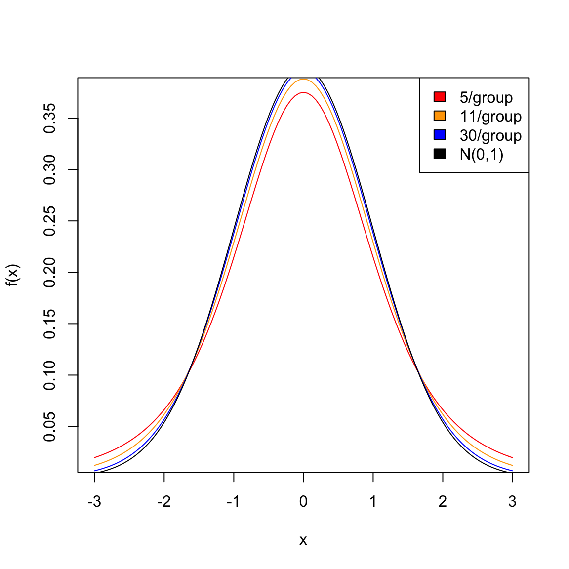
You can see that the \(t\) distribution is like the normal, only it has larger “tails” than the normal, meaning seeing large values is more likely than in a normal distribution.
What happens as you change the sample size?
Notice that if you have largish datasets (e.g. \(>30-50\) samples in each group) then you can see that the t-distribution is numerically almost equivalent to using the normal distribution, so that’s why it’s usually fine to just use the normal distribution to get p-values. Only in small samples sizes are there large differences.
Degrees of Freedom
The t-distribution has one additional parameter called the degrees of freedom, often abreviated as df. This parameter has nothing to do with the mean or standard deviation of the data (since our t-statistic is already standardized), and depends totally on the sample size of our populations. The actual equation for the degrees of freedom is quite complicated: \[df=\frac{\left( \frac{\hat{\sigma}_1^2}{n_1} + \frac{\hat{\sigma}_2^2}{n_2}\right)^2}{\frac{(\frac{\hat{\sigma}_1^2}{n_1})^2}{n_1-1} + \frac{(\frac{\hat{\sigma}_2^2}{n_2})^2}{n_2-1}}.\] This is not an equation you need to learn or memorize, as it is implemented in R for you. A easy approximation for this formula is to use \[df\approx min(n_1-1, n_2-1)\] This approximation is mainly useful to try to understand how the degrees of freedom are changing with your sample size. Basically, the size of the smaller group is the important one. Having one huge group that you compare to a small group doesn’t help much – you will do better to put your resources into increasing the size of the smaller group (in the actual formula it helps a little bit more, but the principle is the same).
3.4.5 Assumptions of the T-test
Parametric tests usually state their assumptions pretty clearly: they assume a parametric model generated the data in order to arrive at the mathematical description of the null distribution. For the t-test, we assume that the data \(X_1,\ldots,X_{n_1}\) and \(Y_1,\ldots,Y_{n_2}\) are normal to get the t-distribution.
What happens if this assumption is wrong? When will it still make sense to use the t-test?
If we didn’t have to estimate the variance, the central limit theorem tells us the normality assumption will work for any distribution, if we have a large enough sample size.
What about the t-distribution? That’s a little tricker. You still need a large sample size; you also need that the distribution of the \(X_i\) and the \(Y_i\), while not required to be exactly normal, not be too far from normal. In particular, you want them to be symmetric (unlike our flight data).22
Generally, the t-statistic is reasonably robust to violations of these assumptions, particularly compared to other parametric tests, if your data is not too skewed and you have a largish sample size (e.g. 30 samples in a group is good). But the permutation test makes far fewer assumptions, and in particular is very robust to assumptions about the distribution of the data.
For small sample sizes (e.g. \(<10\) in each group), you certainly don’t really have any good justification to use the t-distribution unless you have a reason to trust that the data is normally distributed (and with small sample sizes it is also very hard to justify this assumption by looking at the data).
3.4.6 Flight Data and Transformations
Let’s consider the flight data. Recall, the t-statistic focuses on the difference in means. Here are the means of the flight delays in the two airlines we have been considering:
##        AA        UA
##  7.728294 12.255649
Why might the difference in the means not be a compelling comparison for the flight delay?
The validity of the t-test depends assumptions about the distribution of the data, and a common way to assess this is to look at the distribution of each of the two groups.
With larger sample sizes there is less worry about the underlying distribution, but very non-normal input data will not do well with the t-test, particularly if the data is skewed, meaning not symmetrically distributed around its mean.
Here is a histogram of the flight delay data:
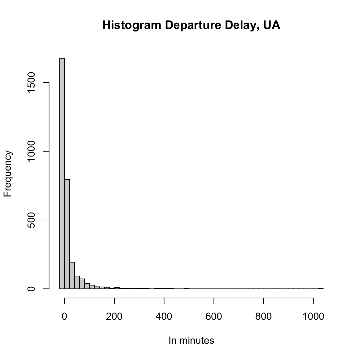
Looking at the histogram of the flight data, would you conclude that the t-test would be a valid choice?
Note that nothing stops us from running the test, whether it is a good idea or not, and it’s a simple one-line code:
t.test(flightSFOSRS$DepDelay[flightSFOSRS$Carrier ==
    "UA"], flightSFOSRS$DepDelay[flightSFOSRS$Carrier ==
    "AA"])
##
## Welch Two Sample t-test
##
## data: flightSFOSRS$DepDelay[flightSFOSRS$Carrier == "UA"] and flightSFOSRS$DepDelay[flightSFOSRS$Carrier == "AA"]
## t = 2.8325, df = 1703.1, p-value = 0.004673
## alternative hypothesis: true difference in means is not equal to 0
## 95 percent confidence interval:
## 1.392379 7.662332
## sample estimates:
## mean of x mean of y
## 12.255649 7.728294This is a common danger of parametric tests. They are implemented everywhere (there are on-line calculators that will compute this for you; excel will do this calculation), so people are drawn to doing this, while permutation tests are more difficult to find pre-packaged.
Direct comparison to the permutation test
The permutation test can use any statistic we like, and the t-statistic is a perfectly reasonable way to compare two distributions if we are interested in comparing the means (though as we mentioned, we might not be!). So we can compare the t-test to a permutation test of the mean using the t-statistic. We implement the permutation test with the t-statistic here:
set.seed(489712)
tstatFun <- function(x1, x2) {
    abs(t.test(x1, x2)$statistic)
}
dataset <- flightSFOSRS
output <- permutation.test(group1 = dataset$DepDelay[dataset$Carrier ==
    "UA"], group2 = dataset$DepDelay[dataset$Carrier ==
    "AA"], FUN = tstatFun, n.repetitions = 10000)
cat("permutation pvalue=", output$p.value)
## permutation pvalue= 0.0076We can also run the t-test again and compare it.
tout <- t.test(flightSFOSRS$DepDelay[flightSFOSRS$Carrier ==
    "UA"], flightSFOSRS$DepDelay[flightSFOSRS$Carrier ==
    "AA"])
cat("t-test pvalue=", tout$p.value)
## t-test pvalue= 0.004673176They don’t result in very different conclusions.
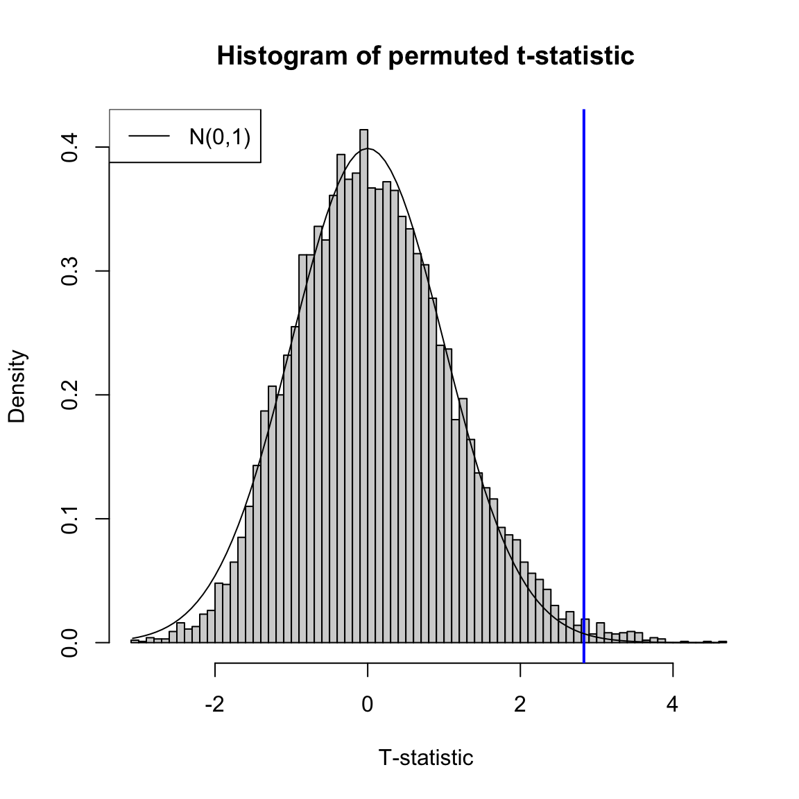
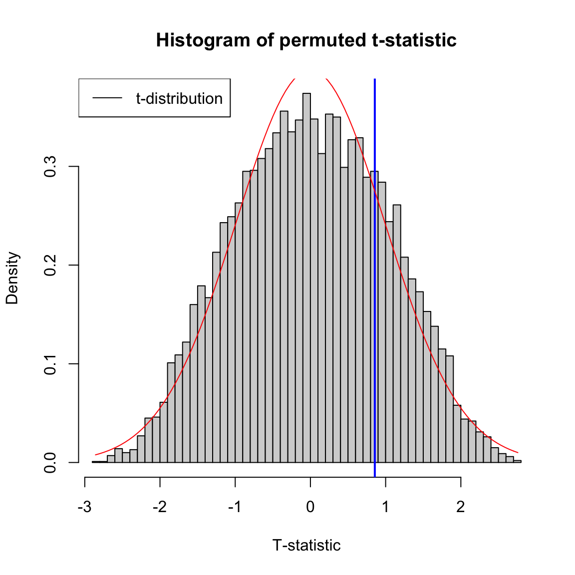
We can compare the distribution of the permutation distribution of the t-statistic, and the density of the \(N(0,1)\) that the parametric model assumes. We can see that they are quite close, even though our data is very skewed and clearly non-normal. Indeed for large sample sizes like we have here, they will often give similar results, even though our data is clearly not meeting the assumptions of the t-test. The t-test really is quite robust to violations.
Smaller Sample Sizes
If we had a smaller dataset we would not get such nice behavior. We can take a sample of our dataset to get a smaller sample of the data of size 20 and 30 in each group. Running both a t-test and a permutation test on this sample of the data, we can see that we do not get a permutation distribution that matches the (roughly) N(0,1) we use for the t-test.
## pvalue permutation= 0.4446## pvalue t.test= 0.394545What different conclusions do you get from the two tests with these smaller datasizes?
Transformations
We saw that skewed data could be problematic in visualization of the data, e.g. in boxplots, and transformations are helpful in this setting. Transformations can also be helpful for applying parametric tests. They can often allow the parametric t-test to work better for smaller datasets.
If we compare both the permutation test and the t-test on log-transformed data, then even with the smaller sample sizes the permutation distribution looks much closer to the t-distribution.
![]()
## pvalue permutation= 0.4446## pvalue t.test= 0.3261271Why didn’t the p-value for the permutation test change?
What does it mean for my null hypothesis to transform to the log-scale? Does this make sense?
3.4.7 Why parametric models?
We do the comparison of the permutation test to the parametric t-test not to encourage the use of the the t-test in this setting – the data, even after transformation, is pretty skewed and there’s no reason to not use the permutation test instead. The permutation test will give pretty similar answers regardless of the transformation23 and is clearly indicated here.
This exercise was to show the use and limits of using the parametric tests, and particularly transformations of the data, in an easy setting. Historically, parametric t-tests were necessary in statistics because there were not computers to run permutation tests. That’s clearly not compelling now! However, it remains that parametric tests are often easier to implement (one-line commands in R, versus writing a function), and you will see parametric tests frequently (even when resampling methods like permutation tests and bootstrap would be more justifiable).
The take-home lesson here regarding parametric tests is that when there are large sample sizes, parametric tests can overcome violations of their assumptions24 so don’t automatically assume parametric tests are completely wrong to use. But a permutation test is the better all-round tool for this question: it is has more minimal assumptions, and can look at how many different statistics we can use.
There are also some important reasons to learn about t-tests, however, beyond a history lesson. They are the easiest example of a parameteric test, where you make assumptions about the distribution your data (i.e. \(X_1,\ldots,X_{n_1}\) and \(Y_{1},\ldots,Y_{n_2}\) are normally distributed). Parametric tests generally are very important, even with computers. Parametric models are particularly helpful for researchers in data science for the development of new methods, particularly in defining good test statistics, like \(T\).
Parametric models are also useful in trying to understand the limitations of a method, mathematically. We can simulate data under different models to understand how a statistical method behaves.
There are also applications where the ideas of bootstrap and permutation tests are difficult to apply. Permutation tests, in particular, are quite specific. Bootstrap methods, which we’ll review in a moment, are more general, but still are not always easy to apply in more complicated settings. A goal of this class is to make you comfortable with parametric models (and their accompanying tests), in addition to the resampling methods you’ve learned.
3.5 Digging into Hypothesis tests
Let’s break down some important concepts as to what makes a test. Note that all of these concepts will apply for any hypothesis test.
- A null hypothesis regarding a particular feature of the data
- A test statistic for which extreme values indicates less correspondence with the null hypothesis
- An assumption of how the data was generated under the null hypothesis
- The distribution of the test statistic under the null hypothesis.
As we’ve seen, different tests can be used to answer the same basic “null” hypothesis – are the two groups “different”? – but the specifics of how that null is defined can be quite different. For any test, you should be clear as to what the answer is to each of these points.
3.5.1 Significance & Type I Error
The term significance refers to measuring how incompatible the data is with the null hypothesis. There are two important terminologies that go along with assessing significance.
- p-values
- You often report a p-value to quantify how unlikely the data is under the null.
- Decision to Reject/Not reject
- Make a final decision as to whether the null hypothesis was too unlikely to have reasonably created the data we’ve seen – either reject the null hypothesis or not.
We can just report the p-value, but it is common to also make an assessment of the p-value and give a final decision as well. In this case we pick a cutoff, e.g. p-value of 0.05, and report that we reject the null.
You might see sentences like “We reject the null at level 0.05.” The level chosen for a test is an important concept in hypothesis testing and is the cutoff value for a test to be significant. In principle, the idea of setting a level is that it is a standard you can require before declaring significance; in this way it can keep researchers from creeping toward declaring significance once they see the data and see they have a p-value of 0.07, rather than 0.05. However, in practice a fixed cutoff value can have the negative result of encouraging researchers to fish in their data until they find something that has a p-value less than 0.05.
Commonly accepted cutoffs for unlikely events are 0.05 or 0.01, but these values are too often considered as magical and set in stone. Reporting the actual p-value is more informative than just saying yes/no whether you reject (rejecting with a p-value of 0.04 versus 0.0001 tells you something about your data).
More about the level
Setting the level of a test defines a repeatable procedure: “reject if p-value is \(< \alpha\)”. The level of the test actually reports the uncertainity in this procedure. Specifically, with any test, you can make two kinds of mistakes:
- Reject the null when the null is true (Type I error)
- Not reject the null when the null is in fact not true (Type II error)
Then the level of a decision is the probability of this procedure making a type I error: if you always reject at 0.05, then 5% of such tests will wrongly reject the null hypothesis when in fact the null is true is true.
Note that this is no different in concept that our previous statement saying that a p-value is the likelihood under the null of an event as extreme as what we observed. However, it does a quantify how willing you are to making Type I Error in setting your cutoff value for decision making.
3.5.2 Type I Error & All Pairwise Tests
Let’s make the importance of accounting and measuring Type I error more concrete. We have been considering only comparing the carriers United and American. But in fact there are 10 airlines.
We might want to compare all of them, in other words run a hypothesis test on each pair of carriers. That’s a hypothesis test for each pair of airlines:
## number of pairs: 45That starts to be a lot of tests. So for speed purposes in class, I’ll use the t-test to illustrate this idea and calculate the t-statistic and its p-value for every pair of airline carriers (with our transformed data):
## [1] 2 45## statistic.t p.value
## AA-AS 1.1514752 0.2501337691
## AA-B6 -3.7413418 0.0002038769
## AA-DL -2.6480549 0.0081705864
## AA-F9 -0.3894014 0.6974223534
## AA-HA 3.1016459 0.0038249362
## AA-OO -2.0305868 0.0424142975## statistic.t p.value
## AA-AS 1.1514752 0.2501337691
## AA-B6 -3.7413418 0.0002038769
## AA-DL -2.6480549 0.0081705864
## AA-F9 -0.3894014 0.6974223534
## AA-HA 3.1016459 0.0038249362
## AA-OO -2.0305868 0.0424142975## Number found with p-value < 0.05: 26 ( 0.58 proportion of tests)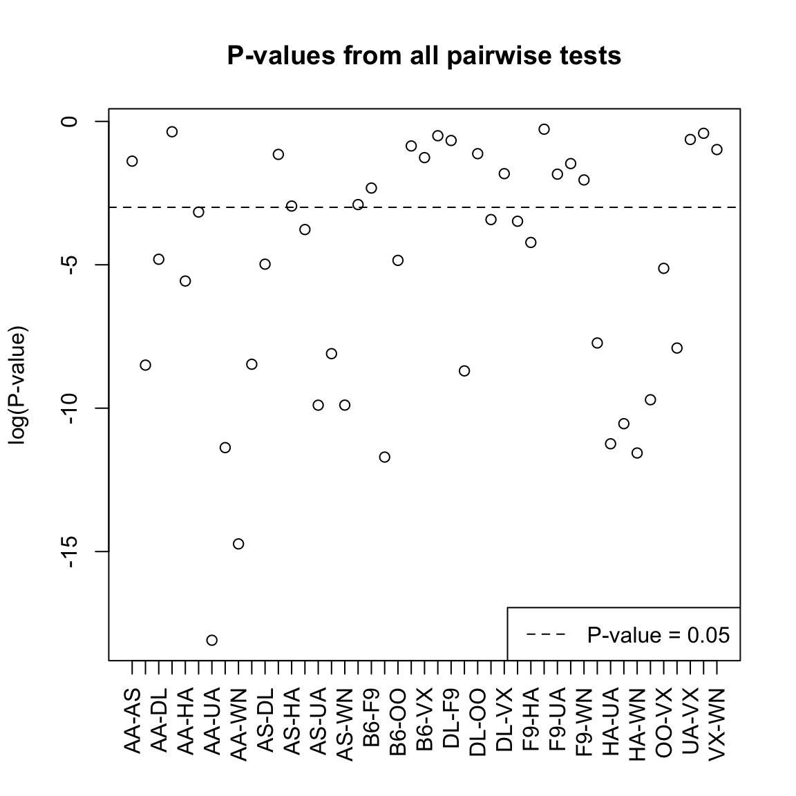
What does this actually mean? Is this a lot to find significant?
Roughly, if each of these tests has level 0.05, then even if none of the pairs are truly different from each other, I might expect on average around 2 to be rejected at level 0.05 just because of variation in sampling.25 This is the danger in asking many questions from your data – something is likely to come up just by chance.26
We can consider this by imagining what if I scramble up the carrier labels – randomly assign a carrier to a flight. Then I know there shouldn’t be any true difference amongst the carriers. I can do all the pairwise tests and see how many are significant.
## Number found with p-value < 0.05: 6 ( 0.13 proportion)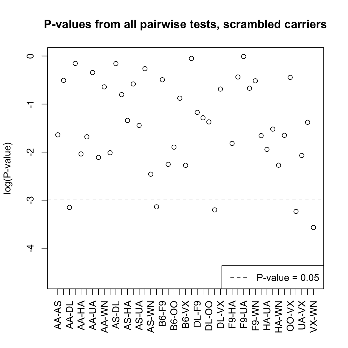
What does this suggest to you about the actual data?
Multiple Testing
Intuitively, we consider that if we are going to do all of these tests, we should have a stricter criteria for rejecting the null so that we do not routinely find pairwise differences when there are none.
Does this mean the level should be higher or lower to get a `stricter’ test? What about the p-value?
Making such a change to account for the number of tests considered falls under the category of multiple testing adjustments, and there are many different flavors beyond the scope of the class. Let’s consider the most widely known correction: the Bonferroni correction.
Specifically, say we will quantify our notion of stricter to require “of all the tests I ran, there’s only a 5% chance of a type I error”. Let’s make this a precise statement. Suppose that of the \(K\) tests we are considering, there are \(V \leq K\) tests that are type I errors, i.e. the null is true but we rejected. We will define our cummulate error rate across the set of \(K\) tests as
\[P(V\geq 1)\]
So we if we can guarantee that our testing procedure for the set of \(K\) tests has \(P(V\geq 1)\leq\gamma\) we have controlled the family-wise error rate to level \(\gamma\).
How to control the family-wise error rate?
We can do a simple correction to our \(K\) individual tests to ensure \(P(V\geq 1)\leq\gamma\). If we lower the level \(\alpha\) we require in order to reject \(H_0\), we will lower our chance of a single type I error, and thus also lowered our family-wise error rate. Specifically, if we run the \(K\) tests and set the individual level of each individualtest to be \(\alpha=\gamma/K\), then we will guarantee that the family-wise error rate is no more than \(\gamma\).
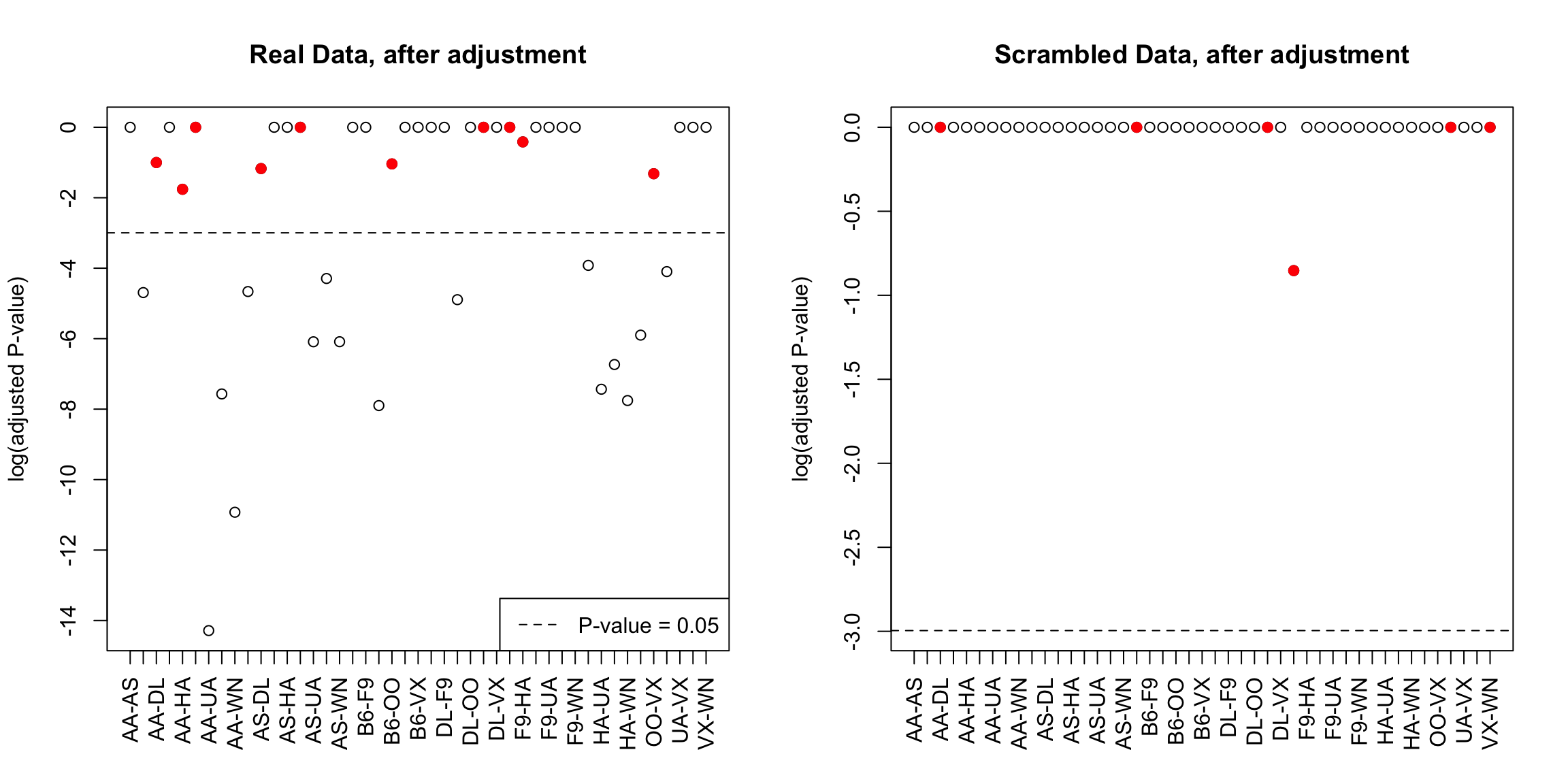
In the example of comparing the different airline carriers, the number of tests is 45. So if we want to control our family-wise error rate to be no more than 0.05, we need each individual tests to reject only with \(\alpha=0.0011\).
## Number found significant after Bonferonni: 16## Number of shuffled differences found significant after Bonferonni: 0If we reject each tests only if \[p-value\leq \alpha=\gamma/K\], then we can equivalently say we only reject if \[K \frac{p-value} \leq \gamma\] We can therefore instead think only about \(\gamma\) (e.g. 0.05), and create adjusted p-values, so that we can just compare our adjusted p-values directly to \(\gamma\). In this case if our standard (single test) p-value is \(p\), we have \[\text{Bonferroni adjusted p-values}= p \times K\]
##       statistic.t      p.value  p.value.adj
## AA-AS   1.1514752 0.2501337691 11.256019611
## AA-B6  -3.7413418 0.0002038769  0.009174458
## AA-DL  -2.6480549 0.0081705864  0.367676386
## AA-F9  -0.3894014 0.6974223534 31.384005904
## AA-HA   3.1016459 0.0038249362  0.172122129
## AA-OO  -2.0305868 0.0424142975  1.908643388
## statistic.t p.value p.value.adj
## AA-AS -1.3008280 0.19388985 8.725043
## AA-B6 0.5208849 0.60264423 27.118990
## AA-DL -2.0270773 0.04281676 1.926754
## AA-F9 -0.1804245 0.85698355 38.564260
## AA-HA -1.5553127 0.13030058 5.863526
## AA-OO -1.3227495 0.18607903 8.373556Notice some of these p-values are greater than 1! So in fact, we want to multiply by \(K\), unless the value is greater than \(1\), in which case we set the p-value to be 1. \[\text{Bonferroni adjusted p-values}= min(p \times K,1)\]
##       statistic.t      p.value  p.value.adj p.value.adj.final
## AA-AS   1.1514752 0.2501337691 11.256019611       1.000000000
## AA-B6  -3.7413418 0.0002038769  0.009174458       0.009174458
## AA-DL  -2.6480549 0.0081705864  0.367676386       0.367676386
## AA-F9  -0.3894014 0.6974223534 31.384005904       1.000000000
## AA-HA   3.1016459 0.0038249362  0.172122129       0.172122129
## AA-OO  -2.0305868 0.0424142975  1.908643388       1.000000000
Now we plot these adjusted values, for both the real data and the data I created by randomly scrambling the labels. I’ve colored in red those tests that become non-significant after the multiple testing correction.
%%%%%%%%%%%%%%%%%%%%%%%%%% %%%%%%%%%%%%%%%%%%%%%%%%%% %%%%%%%%%%%%%%%%%%%%%%%%%% %%%%%%%%%%%%%%%%%%%%%%%%%% %%%%%%%%%%%%%%%%%%%%%%%%%%
3.6 Confidence Intervals
Another approach to inference is with confidence intervals. Confidence intervals give a range of values (based on the data) that are most likely to overlap the true parameter. This means confidence intervals are only appropriate when we are focused on estimation of a specific numeric feature of a distribution (a parameter of the distribution), though they do not have to require parametric models to do so.27
Form of a confidence interval
Confidence intervals also do not rely on a specific null hypothesis; instead they give a range of values (based on the data) that are most likely to overlap the true parameter. Confidence intervals take the form of an interval, and are paired with a confidence, like 95% confidence intervals, or 99% confidence intervals.
Which should should result in wider intervals, a 95% or 99% interval?
General definition of a Confidence interval
A 95% confidence interval for a parameter \(\theta\) is a interval \((V_1, V_2)\) so that \[P(V_1 \leq \theta \leq V_2)=0.95.\] Notice that this equation looks like \(\theta\) should be the random quantity, but \(\theta\) is a fixed (and unknown) value. The random values in this equation are actually the \(V_1\) and \(V_2\) – those are the numbers we estimate from the data. It can be useful to consider this equation as actually, \[P(V_1 \leq \theta \text{ and } V_2 \geq \theta)=0.95,\] to emphasize that \(V_1\) and \(V_2\) are the random variables in this equation.
3.6.1 Quantiles
Without even going further, it’s clear we’re going to be inverting our probability calculations, i.e. finding values that give us specific probabilities. For example, you should know that for \(X\) distributed as a normal distribution, the probability of \(X\) being within about 2 standard deviations of the mean is 0.95 – more precisely 1.96 standard deviations.
Figuring out what number will give you a certain probability of being less than (or greater than) that value is a question of finding a quantile of the distribution. Specifically, quantiles tell you at what point you will have a particular probability of being less than that value. Precisely, if \(z\) is the \(\alpha\) quantile of a distribution, then \[P(X\leq z)=\alpha.\] We will often write \(z_{\alpha}\) for the \(\alpha\) quantile of a distribution.
So if \(X\) is distributed as a normal distribution and \(z\) is a 0.25 quantile of a normal distribution, \[P(X \leq z)=0.25.\] \(z\) is a 0.90 quantile of a normal if \(P(X\leq z)=0.90\), and so forth
These numbers can be looked up easily in R for standard distributions.
## [1] -0.8416212## [1] 1.281552## [1] -1.918876What is the probability of being between -0.84 and 1.2815516 in a \(N(0,1)\)?
3.7 Parametric Confidence Intervals
This time we will start with using parametric models to create confidence intervals. We will start with how to construct a parametric CI for the mean of single group.
3.7.1 Confidence Interval for Mean of One group
As we’ve discussed many times, a SRS will have a sampling distribution that is roughly a normal distribution (the Central Limit Theorem). Namely, that if \(X_1,\ldots,X_n\) are a i.i.d from a distribution with mean \(\mu\) and variance \(\sigma^2\), then \(\hat{\mu}=\bar{X}=\frac{1}{n}\sum_{i=1}^n X_i\) will have a roughly normal distribution \[N(\mu,\frac{\sigma^2}{n}).\]
Let’s assume we know \(\sigma^2\) for now. Then a 95% confidence interval can be constructed by \[\bar{X}\pm 1.96 \frac{\sigma}{\sqrt{n}}\] More generally, we can write this as \[\bar{X}\pm z SD(\bar{X})\]
Where did \(z=1.96\) come from?
Note for a r.v. \(Y\sim N(\mu,\sigma^2)\) distribution, the value \(\mu-1.96\sqrt{\sigma^2}\) is the 0.025 quantile of the distribution, and \(\mu+1.96\sqrt{\sigma^2}\) is the 0.975 quantile of the distribution, so the probability of \(Y\) being between these two values is 0.95. By the CLT we’ll assume \(\bar{X}\sim N(\mu,\frac{\sigma^2}{n})\), so the the probability that \(\bar{X}\) is within \[\mu\pm1.96\sqrt{\sigma^2}\] is 95%. So it looks like we are just estimating \(\mu\) with \(\bar{X}\).
That isn’t quite accurate. What we are saying is that \[P(\mu-1.96\sqrt{\frac{\sigma^2}{n}}\leq \bar{X} \leq \mu+1.96\sqrt{\frac{\sigma^2}{n}})=0.95\]
and we really need is to show that \[P(\bar{X}-1.96\sqrt{\frac{\sigma^2}{n}}\leq \mu \leq \bar{X}+1.96\sqrt{\frac{\sigma^2}{n}})=0.95\] to have a true 0.95 confidence interval. But we’re almost there.
We can invert our equation above, to get \[\begin{align*} 0.95&=P(\mu-1.96\sqrt{\frac{\sigma^2}{n}}\leq \bar{X}\leq \mu+1.96\sqrt{\frac{\sigma^2}{n}})\\ &=P(-1.96\sqrt{\frac{\sigma^2}{n}}\leq \bar{X} -\mu \leq 1.96\sqrt{\frac{\sigma^2}{n}})\\ &=P(-1.96\sqrt{\frac{\sigma^2}{n}}-\bar{X}\leq -\mu \leq 1.96\sqrt{\frac{\sigma^2}{n}}-\bar{X})\\ &=P(1.96\sqrt{\frac{\sigma^2}{n}}+\bar{X}\geq \mu \geq -1.96\sqrt{\frac{\sigma^2}{n}}+\bar{X})\\ &=P(\bar{X}-1.96\sqrt{\frac{\sigma^2}{n}}\leq \mu \leq \bar{X}+1.96\sqrt{\frac{\sigma^2}{n}})\\ \end{align*}\]
General equation for CI
Of course, we can do the same thing for any confidence level we want. If we want a \((1-\alpha)\) level confidence interval, then we take \[\bar{X}\pm z_{\alpha/2} SD(\bar{X})\] Where \(z_{\alpha/2}\) is the \(\alpha/2\) quantile of the \(N(0,1)\).
In practice, we do not know \(\sigma\) so we don’t know \(SD(\bar{X})\) and have to use \(\hat{\sigma}\), which mean that we need to use the quantiles of a \(t\)-distribution with \(n-1\) degrees of freedom for smaller sample sizes.
Example in R
For the flight data, we can get a confidence interval for the mean of the United flights using the function t.test again. We will work on the log-scale, since we’ve already seen that makes more sense for parametric tests because our data is skewed:
##
##  One Sample t-test
##
## data:  log(flightSFOSRS$DepDelay[flightSFOSRS$Carrier == "UA"] + addValue)
## t = 289.15, df = 2964, p-value < 2.2e-16
## alternative hypothesis: true mean is not equal to 0
## 95 percent confidence interval:
##  3.236722 3.280920
## sample estimates:
## mean of x
##  3.258821
Notice the result is on the (shifted) log scale! Because this is a monotonic function, we can invert this to see what this implies on the original scale:
logT <- t.test(log(flightSFOSRS$DepDelay[flightSFOSRS$Carrier ==
    "UA"] + addValue))
exp(logT$conf.int) - addValue
## [1] 3.450158 4.600224
## attr(,"conf.level")
## [1] 0.953.7.2 Confidence Interval for Difference in the Means of Two Groups
Now lets consider the average delay time between the two airlines. Then the parameter of interest is the difference in the means: \[\delta=\mu_{United}-\mu_{American}.\] Using the central limit theorem again, \[\bar{X}-\bar{Y}\sim N(\mu_1-\mu_2, \frac{\sigma_1^2}{n_1}+\frac{\sigma_2^2}{n_2})\]
You can do the same thing for two groups in terms of finding the confidence interval: \[P((\bar{X}-\bar{Y})-1.96 \sqrt{\frac{\sigma_1^2}{n_1}+\frac{\sigma_2^2}{n_2}} \leq \mu_1-\mu_2 \leq (\bar{X}-\bar{Y})+1.96\sqrt{\frac{\sigma_1^2}{n_1}+\frac{\sigma_2^2}{n_2}})=0.95\]
Then a 95% confidence interval for \(\mu_1-\mu_2\) if we knew \(\sigma^2_1\) and \(\sigma_2^2\) is \[\bar{X}-\bar{Y}\pm 1.96 \sqrt{\frac{\sigma_1^2}{n_1}+\frac{\sigma_2^2}{n_2}}\]
Estimating the variance
Of course, we don’t know \(\sigma^2_1\) and \(\sigma_2^2\), so we will estimate them, as with the t-statistic. We know from our t-test that if \(X_1,\ldots,X_{n_1}\) and \(Y_1,\ldots,Y_{n_2}\) are normally distributed, then our t-statistic, \[T=\frac{|\bar{X}-\bar{Y}|}{\sqrt{\frac{\hat{\sigma_1}^2}{n_1}+\frac{\hat{\sigma_2}^2}{n_2}}}.\] has actually a t-distribution.
How does this get a confidence interval (T is not an estimate of \(\delta\))? We can use the same logic of inverting the equations, only with the quantiles of the t-distribution to get a confidence interval for the difference.
Let \(t_{0.025}\) and \(t_{0.975}\) be the quantiles of the t distribution. Then, \[P((\bar{X}-\bar{Y})-t_{0.975} \sqrt{\frac{\sigma_1^2}{n_1}+\frac{\sigma_2^2}{n_2}} \leq \mu_1-\mu_2 \leq (\bar{X}-\bar{Y})-t_{0.025}\sqrt{\frac{\sigma_1^2}{n_1}+\frac{\sigma_2^2}{n_2}})=0.95\] Of course, since the \(t\) distribution is symmetric, \(- t_{0.025}=t_{0.975}\).
Why does symmetry imply that \(- t_{0.025}=t_{0.975}\)?
We’ve already seen that for reasonably moderate sample sizes, the difference between the normal and the t-distribution is not that great, so that in most cases it is reasonable to use the normal-based confidence intervals only with \(\hat{\sigma}_1^2\) and \(\hat{\sigma}_2^2\). This is why \(\pm 2\) standard errors is such a common mantra for reporting estimates.
2-group test in R
We can get the confidence interval for the difference in our groups using t.test as well.
logUA <- log(flightSFOSRS$DepDelay[flightSFOSRS$Carrier ==
    "UA"] + addValue)
logAA <- log(flightSFOSRS$DepDelay[flightSFOSRS$Carrier ==
    "AA"] + addValue)
t.test(logUA, logAA)
##
## Welch Two Sample t-test
##
## data: logUA and logAA
## t = 5.7011, df = 1800.7, p-value = 1.389e-08
## alternative hypothesis: true difference in means is not equal to 0
## 95 percent confidence interval:
## 0.07952358 0.16293414
## sample estimates:
## mean of x mean of y
## 3.258821 3.137592What is the problem from this confidence interval on the log-scale that we didn’t have before when we were looking at a single group?
3.8 Bootstrap Confidence Intervals
The Setup
Suppose we are interested instead in whether the median of the two groups is the same.
Why might that be a better idea than the mean?
Or, alternatively, as we saw, perhaps a more relevant statistic than either the mean or the median would be the difference in the proportion greater than 15 minutes late. Let \(\theta_{United}\), and \(\theta_{American}\) be the true proportions of the two groups, and now \[\delta=\theta_{United}-\theta_{American}.\]
The sample statistic estimating \(\delta\) would be what?
To be able to do hypothesis testing on other statistics, we need the distribution of our test statistic to either construct confidence intervals or the p-value. In the t-test, we used the central limit theorem that tells us the difference in the means is approximately normal. We can’t use the CLT theory for the median, however, because the CLT was for the difference in the means of the groups. We would need to have new mathematical theory for the difference in the medians or proportions. In fact such theory exists (and the proportion is actually a type of mean, so we can in fact basically use the t-test, which some modifications). Therefore, many other statistics can also be handled with parametric tests as well, but each one requires a new mathematical theory to get the null distribution. More importantly, when you go with statistics that are beyond the mean, the mathematics often require more assumptions about the data-generating distribution – the central limit theorem for the mean works for most any distribution you can imagine (with large enough sample size), but that’s a special property of the mean. Furthermore, if you have an uncommon statistic, the mathematical theory for the statistic may not exist.
Another approach is to try to estimate the distribution of our test-statistic from our data. This is what the bootstrap does. We’ve talked about estimating the distribution of our data in Chapter 2, but notice that estimating the distribution of our data is a different question than estimating the distribution of a summary statistic. If our data is i.i.d. from the same distribution, then we have \(n\) observations from the distribution from which to estimate the data distribution. For our test statistic (e.g. the median or mean) we have only 1 value. We can’t estimate a distribution from a single value!
The bootstrap is a clever way of estimating the distribution of most any statistic from the data.
3.8.1 The Main Idea: Create many datasets
Let’s step back to some first principles. Recall for a confidence interval based on my statistic \(\delta\), I would like to find numbers \(w_1\) and \(w_2\) so that \[0.95=P(\hat\delta-w_1\leq \delta \leq \hat\delta+w_2)\] so that I would have a CI \(( V_1=\hat\delta-w_1, V_2=\hat\delta+w_2)\).
Note that this is the same as \[P(\delta-w_2\leq \hat{\delta} \leq \delta+w_1)\] In other words, if I knew \(\hat\delta\) had following distribution/density, I could find quantiles that gave me my \(w_1\),\(w_2\).
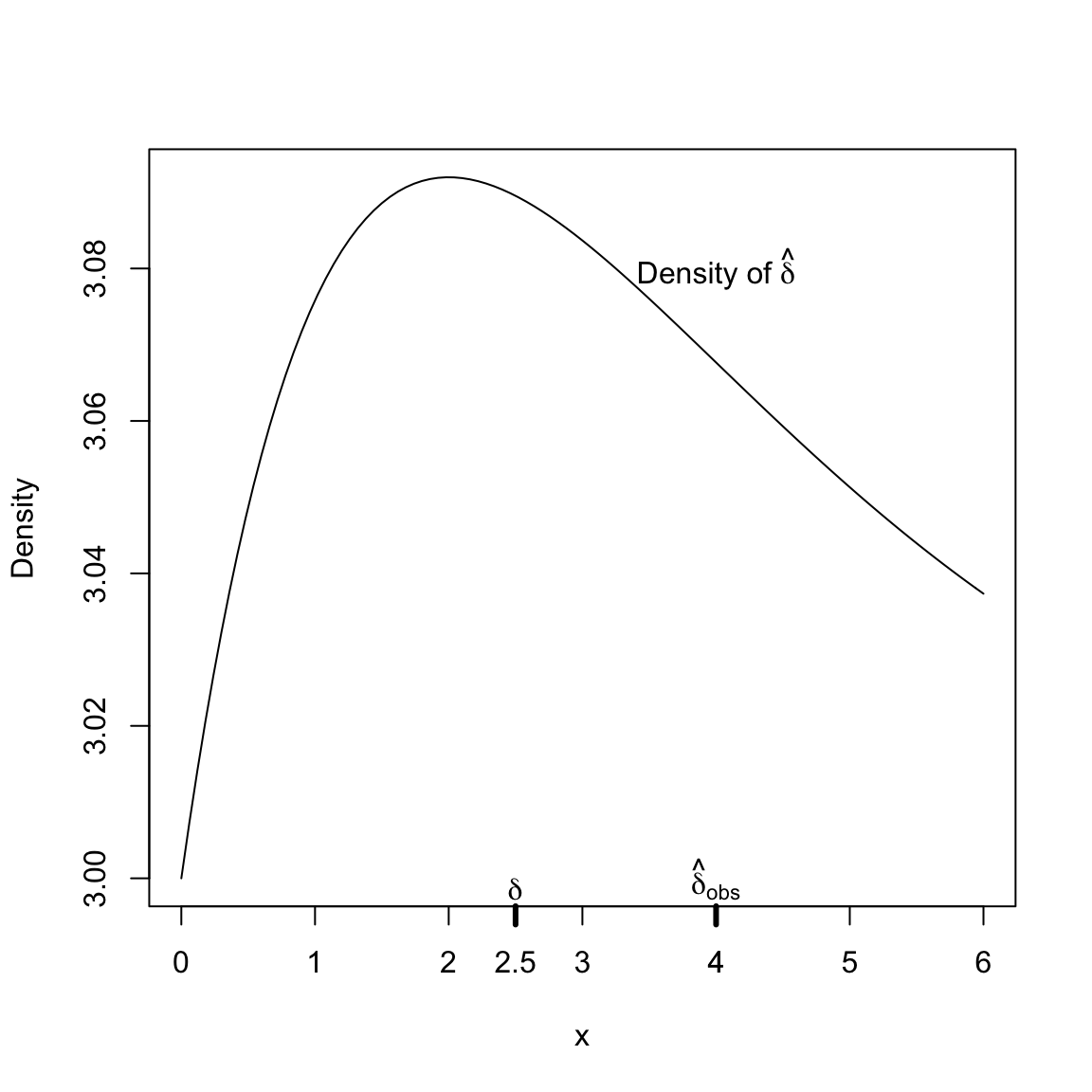
In order to get the distribution of \(\hat{\delta}\), we would like to be able to do is collect multiple data sets, and for each data set calculate our \(\hat{\delta}\). This would give us a collection of \(\hat{\delta}\) from which we could estimate the distribution of \(\hat{\delta}\). More formally, if we knew \(F, G\) – the distributions of the data in each group – we could simulate datasets from each distribution, calculate \(\hat{\delta}\), and repeat this over and over. From each of these multiple datasets, we would calculate \(\hat{\delta}\), which would give us a distribution of \(\hat{\delta}\). This process is demonstrated in this figure:

But since we have only one data set, we only see one \(\hat{\delta}\), so none of this is an option.
What are our options? We’ve seen one option is to use parametric methods, where the distribution of \(\hat{\delta}\) is determined mathematically (but is dependent on our statistic \(\delta\) and often with assumptions about the distributions \(F\) and \(G\)). The other option we will discuss, the bootstrap, tries instead to create lots of datasets with the computer.
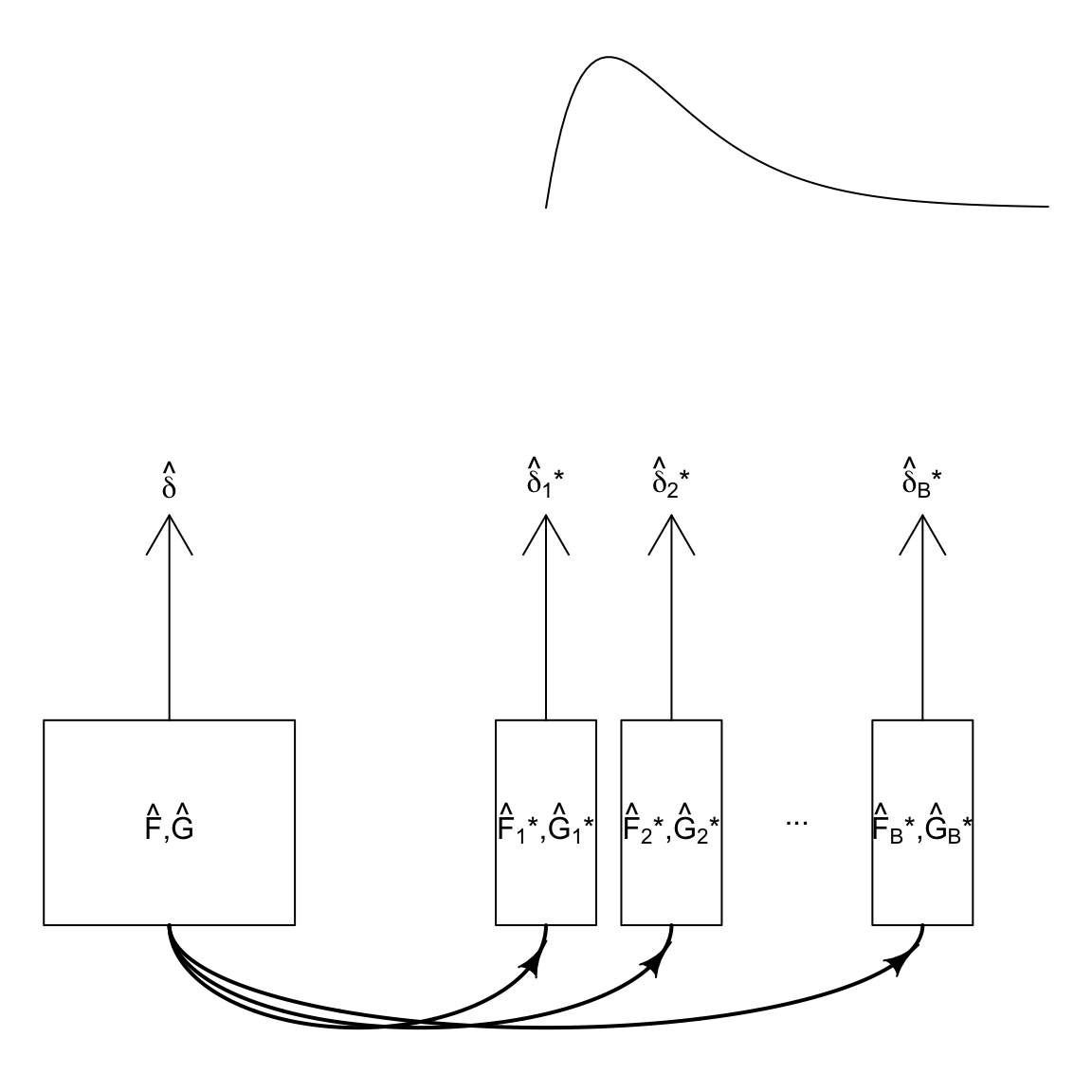
The idea of the bootstrap is if we can estimate the distributions \(F\) and \(G\) with \(\hat{F}\) and \(\hat{G}\), we can create new data sets by simulating data from \(\hat{F}\) and \(\hat{G}\). So we can do our ideal process described above, only without the true \(F\) and \(G\), but with an estimate of them. In other words, while what we need is the distribution of \(\hat{\delta}\) from many datasets from \(F,G\), instead we will create many datasets from \(\hat{F}, \hat{G}\) as an approximation.
Here is a visual of how we are trying to replicate the process with our bootstrap samples:
How can we estimate \(\hat{F},\hat{G}\)? Well, that’s what we’ve discussed in the Chapter 2. Specifically, when we have a i.i.d sample, Chapter 2 went over methods of estimating the unknown true distribution \(F\), and estimating probabilities from \(F\). What we need here is a simpler question – how to draw a sample from an estimate of \(\hat{F}\), which we will discuss next.
Assume we get a i.i.d. sample from \(F\) and \(G\). We’ve previously estimated for example, the density of our distribution (which then defines the entire distribution). But right now, we really need to be able to draw a random sample \(X_1,\ldots,X_{n_1}\) and \(Y_1,\ldots,Y_{n_2}\) from our estimates of the distribution so we can calculate a \(\delta\). Our density estimate doesn’t give us a way to do that.
So we are going to think how can we get an estimate of \(F\) and \(G\) that we can get a sample from? We’ve seen how a full census of our data implies a distribution, if we assume random independent draws from that full data. In other words, a data set combined with a mechanism for drawing samples defines a distribution, with probabilities, etc. So our observed sample gives us an estimated distribution (also called the empirical distribution) \(\hat{F}\) and \(\hat{G}\) from which we can draw samples.
How would you make a i.i.d. sample from your data?
Let \(X_1^*,\ldots, X_{n_1}^*\) be i.i.d. draws from my observed data. This is called a bootstrap sample. I can calculate \(\delta\) from this data, call it \(\hat\delta^*\). Unlike the \(\hat\delta\) from my actual data, I can repeat the process and calculate many \(\hat\delta^*\) values. If I do this enough I have a distribution of \(\hat\delta^*\) values, which we will call the bootstrap distribution of \(\delta\). So the bootstrap distribution of \(\hat\delta\) is the distribution of \(\hat\delta\) if the data was drawn from \(\hat{F}\) and \(\hat{G}\) distribution.
Another funny thing is that \(\hat\delta^*\) is an estimate of \(\hat{\delta}\), i.e. if I didn’t know \(\hat{F}, \hat{G}\) and only saw the bootstrap sample \(X_1^*,\ldots, X_{n_1}^*\) and \(Y_1^*,\ldots, Y_{n_2}^*\), \(\hat\delta^*\) is an estimate of \(\hat{\delta}\). Of course I don’t need to estimate \(\hat{\delta}\) – I know them from my data! But my bootstrap sample can give me an idea of how good of an estimate I can expect \(\hat{\delta}\) to be. If the distribution of \(\hat\delta^*\) shows that we are likely to get estimates of \(\hat\delta\) is far from \(\hat\delta\), then it is likely that \(\hat\delta\) is similarly far from the unknown \(\delta\). It’s when we have simulated data to see what to expect the behavior of our statistic compared to the truth (only now our observed data and \(\hat\delta\) are our ``truth").
Back to Confidence Intervals
If draw many bootstrap samples, I can get the following distribution of \(\hat{\delta}^*\) (centered now at \(\hat{\delta}\)!):
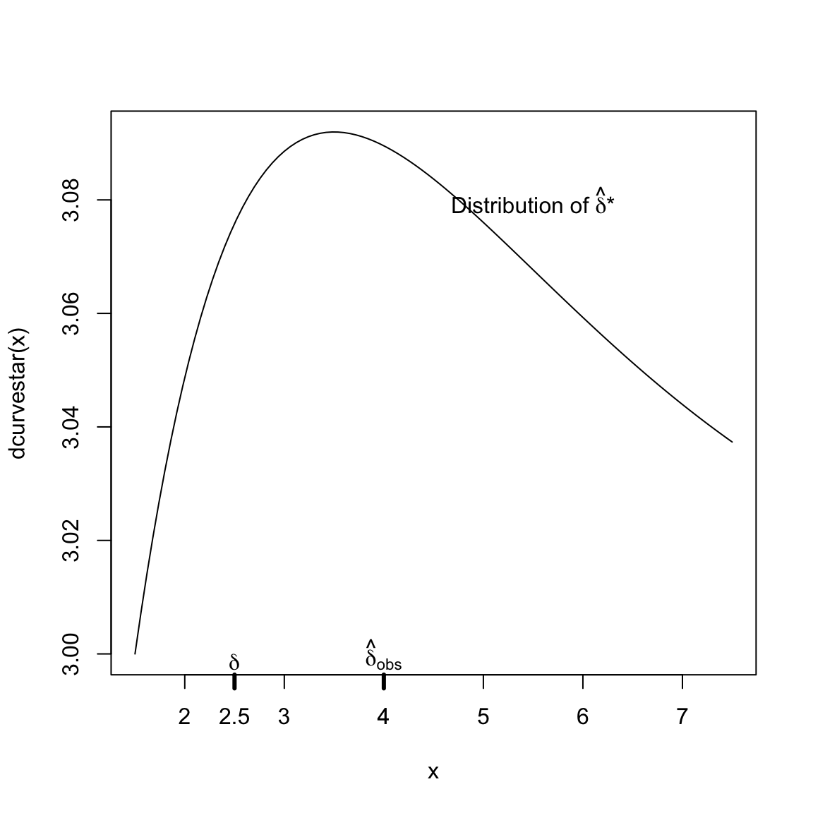
So \(\hat{\delta}^*\) is not a direct estimate of the distribution of \(\hat{\delta}\)! The true distribution of \(\hat\delta\) should be centered at \(\delta\) (and we know \(\hat\delta\neq \delta\) because of randomness). So the bootstrap distribution is NOT the distribution of \(\hat\delta\)
But if the distribution of \(\hat{\delta}^*\) around \(\hat{\delta}\) is like that of \(\hat{\delta}\) around \(\delta\), then that gives me useful information about how likely it is that my \(\hat{\delta}\) is far away from the true \(\delta\), e.g. \[P(|\hat{\delta}-\delta| > 1) \approx P(|\hat{\delta}^*-\hat{\delta}| > 1)\]
Or more relevant for a confidence interval, I could find \(W_1^*\) and \(W_2^*\) so that \[0.95=P(\hat{\delta}-W_2^*\leq \hat{\delta}^* \leq \hat{\delta}+W_1^*)\] Once I found those values, I could use the same \(W_1^*\), \(W_2^*\) to approximate that \[0.95\approx P(\delta-W_2^*\leq \hat{\delta} \leq \delta+W_1^*)=P(\hat\delta-W_1^*\leq \delta \leq \hat\delta+W_2^*)\] This gives us a confidence interval \((\hat\delta-W_1^*, \hat\delta+W_2^*)\) which is called the bootstrap confidence interval for \(\delta\).
In short, we don’t need that \(\hat{\delta}^*\) approximates the distribution of \(\hat{\delta}\). We just want that the distance of \(\hat{\delta}^*\) from it’s true generating value \(\hat{\delta}\) replicate the distance of \(\hat{\delta}\) from the (unknown) true generating value \(\delta\).
3.8.2 Implementing the bootstrap confidence intervals
What does it actually mean to resample from \(\hat{F}\)? It means to take a sample from \(\hat{F}\) just like the kind of sample we took from the actual data generating process, \(F\).
Specifically in our two group setting, say we assume we have a i.i.d sample \(X_1,\ldots,X_{n_1},Y_1,\ldots,Y_{n_2}\) from an unknown distributions \(F\) and \(G\).
What does this actually mean? Consider our airline data; if we took the full population of airline data, what are we doing to create a i.i.d sample?
Then to recreate this we need to do the exact same thing, only from our sample. Specifically, we resample with replacement to get a single bootstrap sample of the same size consisting of new set of samples, \(X_1^*,\ldots,X_{n_1}^*\) and \(Y_1^*,\ldots,Y_{n_2}^*\). Every value of \(X_i^*\) and \(Y_i^*\) that I see in the bootstrap sample will be a value in my original data.
Moreover, some values of my data I will see more than once, why?
From this single bootstrap sample, we can recalculate the difference of the medians on this sample to get \(\hat{\delta}^*.\)
We do this repeatedly, and get a distribution of \(\hat{\delta}^*\); specifically if we repeat this \(B\) times, we will get \(\hat{\delta}^*_1,\ldots,\hat{\delta}_B^*\). So we will now have a distribution of values for \(\hat{\delta}^*\).
We can apply this function to the flight data, and examine our distribution of \(\hat{\delta}^*\).
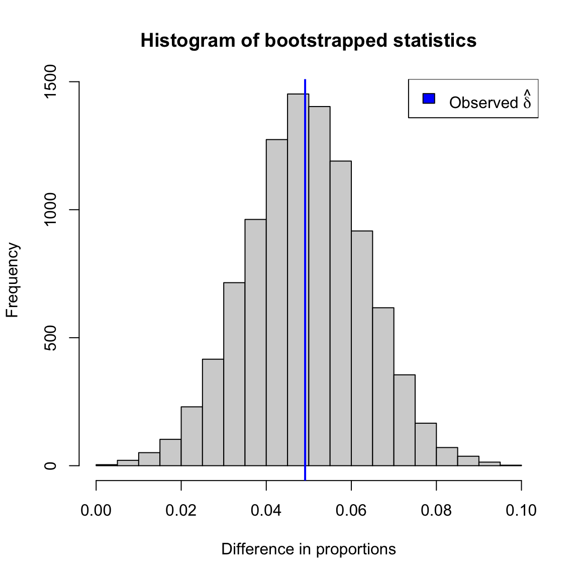
To construct a confidence interval, we use the 0.025 and 0.975 quantiles as the limits of the 95% confidence interval.28 We apply it to our flight data set to get a confidence interval for the difference in proportion of late or cancelled flights.
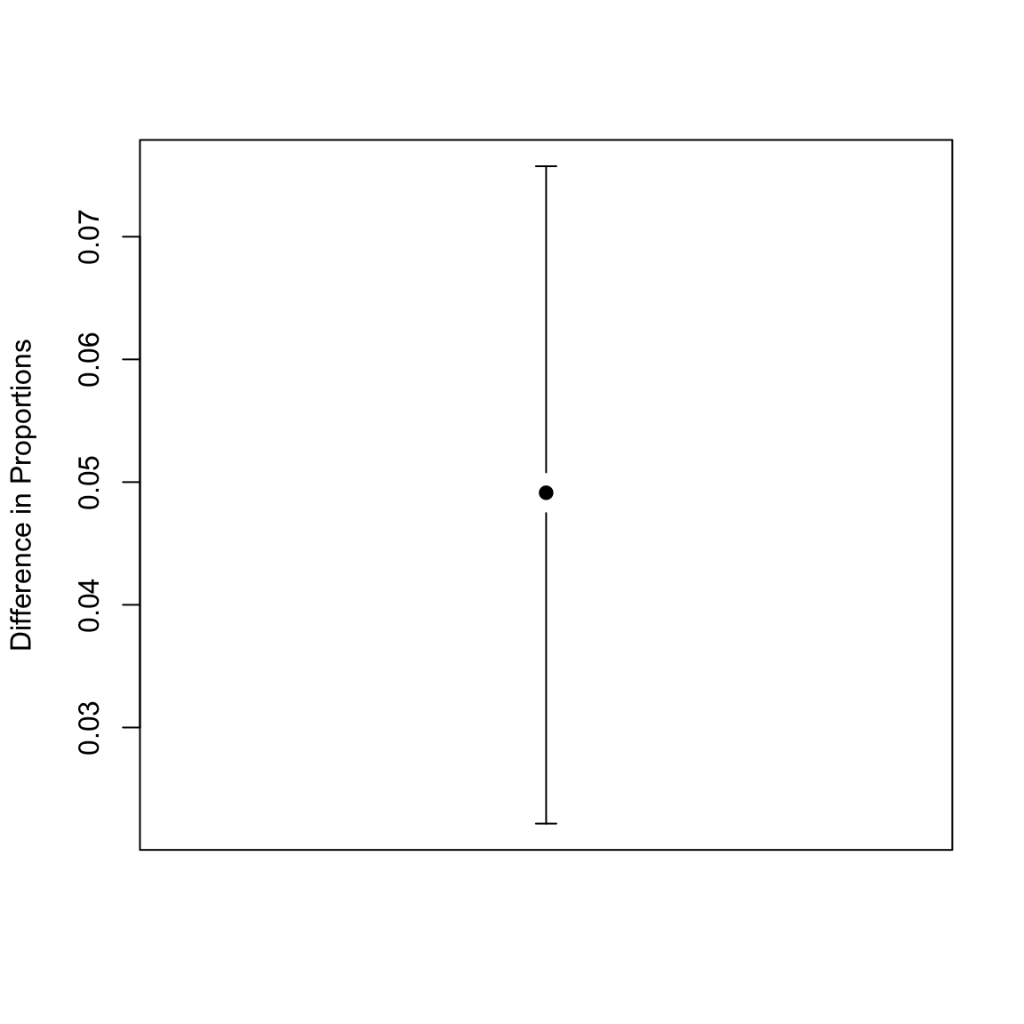
How do you interpret this confidence interval?
3.8.3 Assumptions: Bootstrap
Assumption: Good estimates of \(\hat{F}\), \(\hat{G}\)
A big assumption of the bootstrap is that our sample distribution \(\hat{F}, \hat{G}\) is a good estimate of \(F\) and \(G\). We’ve already seen that will not necessarily the case. Here are some examples of why that might fail:
- Sample size \(n_1\)/\(n_2\) is too small
- The data is not i.i.d sample (or SRS)
Assumption: Data generation process
Another assumption is that our method of generating our data \(X_i^*\), and \(Y_i^*\) matches the way \(X_i\) and \(Y_i\) were generated from \(F,G\). In particular, in the bootstrap procedure above, we are assuming that \(X_i\) and \(Y_i\) are i.i.d from \(F\) and \(G\) (i.e. a SRS with replacement).
Assumption: Well-behaved test statistic
We also need that the parameter \(\theta\) and the estimate \(\hat{\theta}\) to be well behaved in certain ways
- \(\hat{\theta}\) needs to be an unbiased estimate of \(\theta\), meaning across many samples, the average of the \(\hat{\theta}\) is equal to the true parameter \(\theta\) 29
- \(\theta\) is a function of \(F\) and \(G\), and we need that the value of \(\theta\) changes smoothly as we change \(F\) and \(G\). In other words if we changed from \(F\) to \(F'\), then \(\theta\) would change to \(\theta'\); we want if our new \(F'\) is very “close” to \(F\), then our new \(\theta'\) would be very close to \(\theta\). This is a pretty mathematical requirement, and requires a precise definition of "close’’ for two distributions that is not too important for this class to understand.
But here’s an example to make it somewhat concrete: if the parameter \(\theta\) you are interested in is the maximum possible value of a distribution \(F\), then \(\theta\) does NOT change smoothly with \(F\). Why? because you can choose distributions \(F'\) that are very close to \(F\) in every reasonable way to compare two distributions, but their maximum values \(\theta\) and \(\theta'\) are very far apart.30
Another bootstrap confidence interval (Optional)
We can actually use the bootstrap to calculate a confidence interval similarly to that of the normal distribution based on estimating the distribution of \(\hat{\delta} -\delta\).
Notice with the previous calculation for \(\bar{X}\), if I know \[0.95=P(1.96\sqrt{\frac{\sigma^2}{n}}\leq \bar{X} -\mu \leq 1.96\sqrt{\frac{\sigma^2}{n}})\] Then I can invert to get \[0.95=P(\bar{X}-1.96\sqrt{\frac{\sigma^2}{n}}\leq \mu \leq \bar{X}-1.96\sqrt{\frac{\sigma^2}{n}}) \]
So more generally, suppose we have points \(z_{0.025}\) and \(z_{0.975}\) so that \[0.95=P(z_{0.025}\leq \hat{\delta} -\delta \leq z_{0.975})\] e.g. the 0.025 and 0.975 quantiles of \(\hat{\delta} -\delta\). Then I can invert to get \[0.95=P(\hat{\delta}-z_{0.975} \leq \delta \leq \hat{\delta}-z_{0.025} )\] So if I can get the quantiles of \(\hat{\delta} -\delta\), I can make a confidence interval.
So we could use the bootstrap to get estimates of the distribution of \(\hat{\delta} -\delta\) instead of the distribution of \(\hat{\delta}\) and use the quantiles of \(\hat{\delta} -\delta\) to get confidence intervals that are \((\hat{\delta}-z_{0.975},\hat{\delta}-z_{0.025})\). This actually gives a different confidence interval, particularly if the distribution of \(\hat{\delta}\) is not symmetric. The earlier method we talked about is called the percentile method, and is most commonly used, partly because it’s easier to generalize than this method.31
3.9 Thinking about confidence intervals
Suppose you have a 95% confidence interval for \(\delta\) given by \((.02,.07)\).
What is wrong with the following statements regarding this confidence interval? - \(\delta\) has a 0.95 probability of being between \((.02,.07)\) - If you repeatedly resampled the data, the difference \(\delta\) would be within \((.02,.07)\) 95% of the time.
Confidence Intervals or Hypothesis Testing?
Bootstrap inference via confidence intervals is more widely applicable than permutation tests we described above. The permutation test relied on being able to simulate from the null hypothesis, by using the fact that if you detach the data from their labels you can use resampling techniques to generate a null distribution. In settings that are more complicated than comparing groups, it can be difficult to find this kind of trick.
Frequently, confidence intervals and hypothesis testing are actually closely intertwined, particularly for parametric methods. For example, for the parametric test and the parametric confidence interval, they both relied on the distribution of the same statistic, the t-statistic. If you create a 95% confidence interval, and then decide to reject a specific null hypothesis (e.g. \(H_0: \delta=0\)) only when it does not fall within the confidence interval, then this will exactly correspond to a test with level 0.05. So the same notions of level, and type I error, also apply to confidence intervals
Confidence intervals, on the other hand, give much greater interpretation and understanding about the parameter.
3.9.1 Comparing Means: CI of means vs CI of difference
We have focused on creating a confidence interval of the difference (\(\delta\)). Another common strategy is to do a confidence interval of each mean, and compare them.
We can compare these two options using the t-statistic:
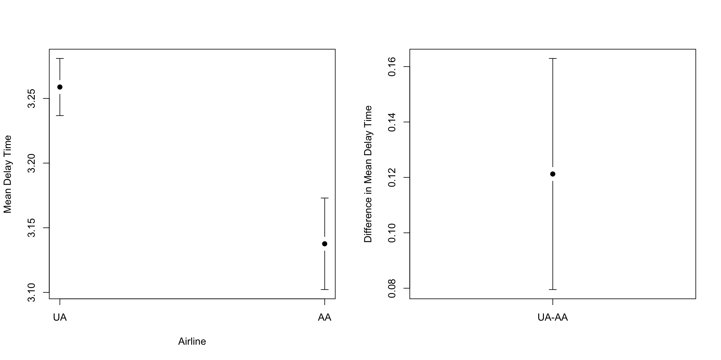
We see that their confidence intervals don’t overlap, and that the CI for the difference in the means doesn’t overlap zero, so we draw the same conclusion in our comparison, namely that the means are different.
However, this doesn’t have to be the case. Here’s some made-up data32:
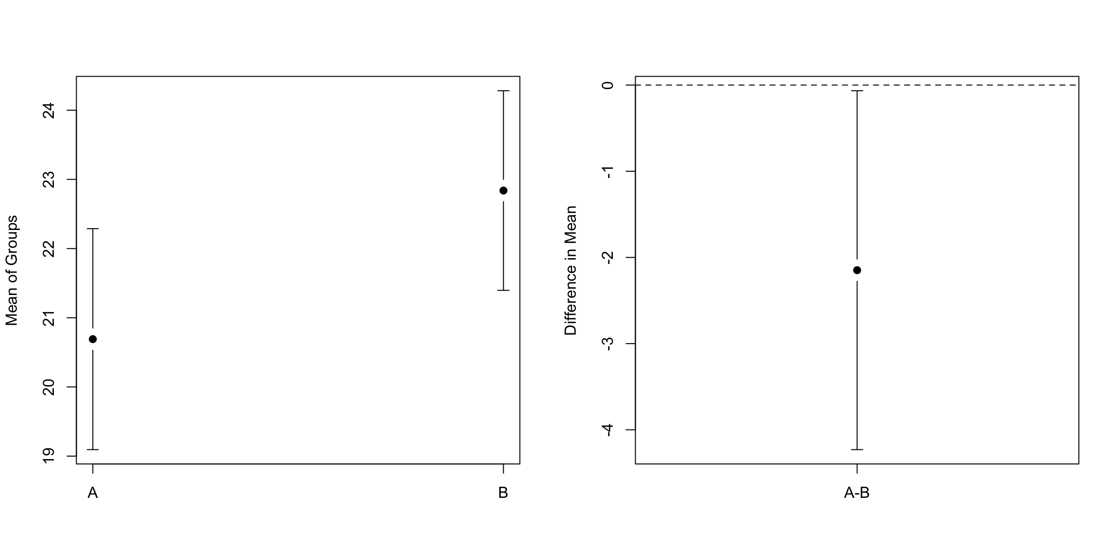
What to think here? What is the right conclusion? The confidence interval for the difference for the means corresponds to the test for the difference of the means, which means that if the CI for \(\delta\) doesn’t cover zero, then the corresponding p-value from the t-test will be \(<0.05\). So this is the “right” confidence interval for determining statistical significance.
Why does this happen?
Basically, with the t-test-based CI, we can examine this analytically (a big advantage of parametric models).
In the first case, for a CI of the difference \(\delta\) to be significantly larger than zero, it means that the lower end of the CI for delta is greater than zero: \[\bar{X}-\bar{Y}> 1.96 \sqrt{\frac{\hat{\sigma}_1^2}{n_1}+\frac{\hat{\sigma}_2^2}{n_2}}\]
Alternatively, if we create the two confidence intervals for \(\bar{X}\) and \(\bar{Y}\), separately, to have them not overlap, we need that the lower end of the CI for \(X\) be greater than the upper end of the CI of \(Y\): \[\begin{align*}\bar{X}-1.96 \sqrt{\frac{\hat{\sigma}_1^2}{n_1}} &> \bar{Y} + 1.96 \sqrt{\frac{\hat{\sigma}_2^2}{n_2}}\\ \bar{X}-\bar{Y}&> 1.96 \left(\sqrt{\frac{\hat{\sigma}_2^2}{n_2}}+ \sqrt{\frac{\hat{\sigma}_1^2}{n_1}}\right) \end{align*}\]
Note that these are not the same requirements. In particular, \[\sqrt{\frac{\hat{\sigma}_1^2}{n_1}+\frac{\hat{\sigma}_2^2}{n_2}} < \left(\sqrt{\frac{\hat{\sigma}_2^2}{n_2}}+ \sqrt{\frac{\hat{\sigma}_1^2}{n_1}}\right)\] (take the square of both sides…).
So that means that the difference of the means doesn’t have to be as big for CI based for \(\delta\) to see the difference as for comparing the individual mean’s CI. We know that the CI for \(\delta\) is equivalent to a hypothesis test, so that means that IF there is a difference between the individual CI means there is a significant difference between the groups, but the converse is NOT true: there could be significant differences between the means of the groups but the CI of the individual means are overlapping.
Reality Check
However, note that the actual difference between the two groups in our toy example is pretty small and our significance is pretty marginal. So it’s not such a big difference in our conclusions after all.
3.10 Revisiting pairwise comparisons
Just as with hypothesis testing, you can have multiple comparison problems with confidence intervals. Consider our pairwise comparisons of the different carriers. We can also create confidence intervals for them all. Again, we will use the t-test on the log-differences to make this go quickly.
##       mean.of.x mean.of.y        lower       upper
## AA-AS  3.086589  3.137592 -0.138045593  0.03603950
## AA-B6  3.289174  3.137592  0.071983930  0.23118020
## AA-DL  3.209319  3.137592  0.018600177  0.12485342
## AA-F9  3.164201  3.137592 -0.108192832  0.16141032
## AA-HA  2.943335  3.137592 -0.321473062 -0.06704092
## AA-OO  3.184732  3.137592  0.001615038  0.09266604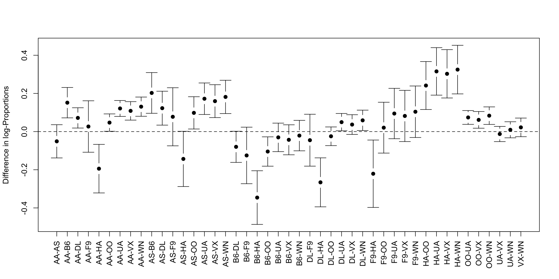
These confidence intervals suffer from the same problem as the p-values: even if the null value (0) is true in every test, roughly 5% of them will happen to not cover 0 just by chance.
So we can do bonferonni corrections to the confidence intervals. Since a 95% confidence interval corresponds to a level 0.05 test, if we go to a \(0.05/K\) level, which is the bonferonni correction, that corresponds to a \(100*(1-0.05/K)\)% confidence interval.
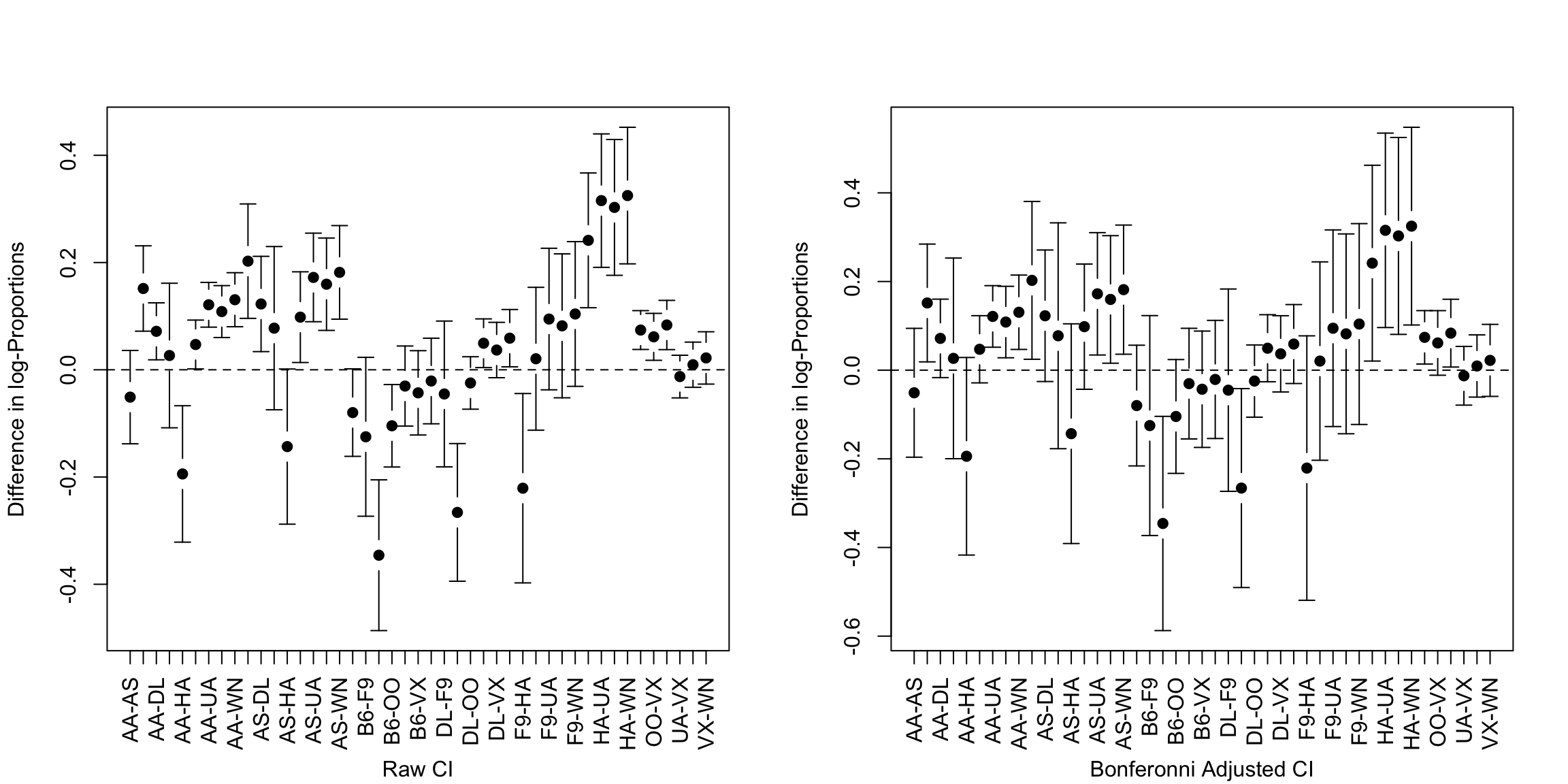
TukeyHSD
In fact, as mentioned, there are many ways to do multiple testing corrections, and Bonferonni is the simplest, yet often most crude correction. There is a multiple testing correction just for pairwise comparisons that use the t-test, called the Tukey HSD test.
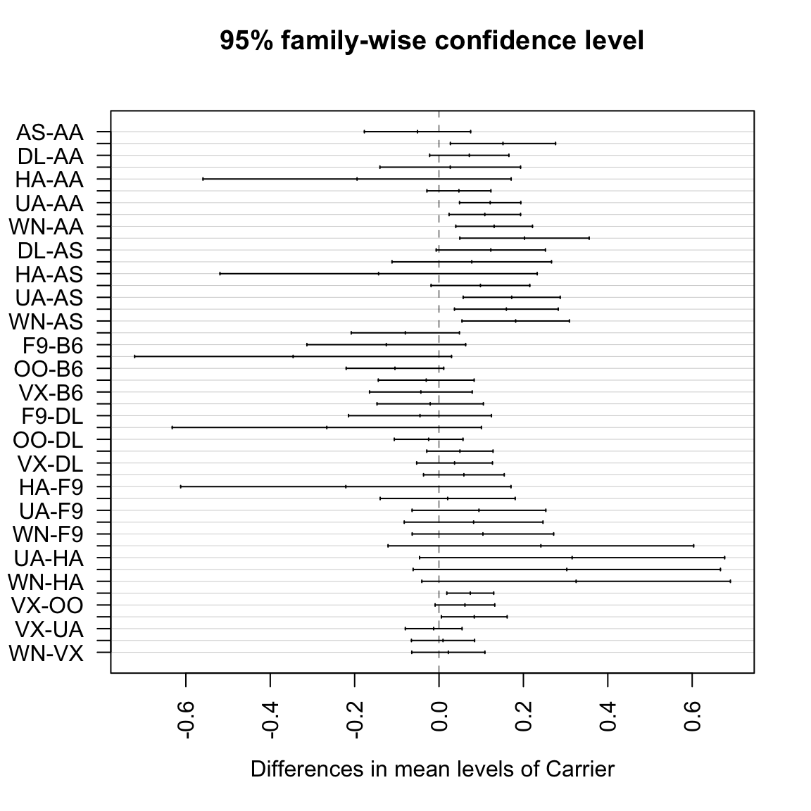 Let’s compare them side-by-side.
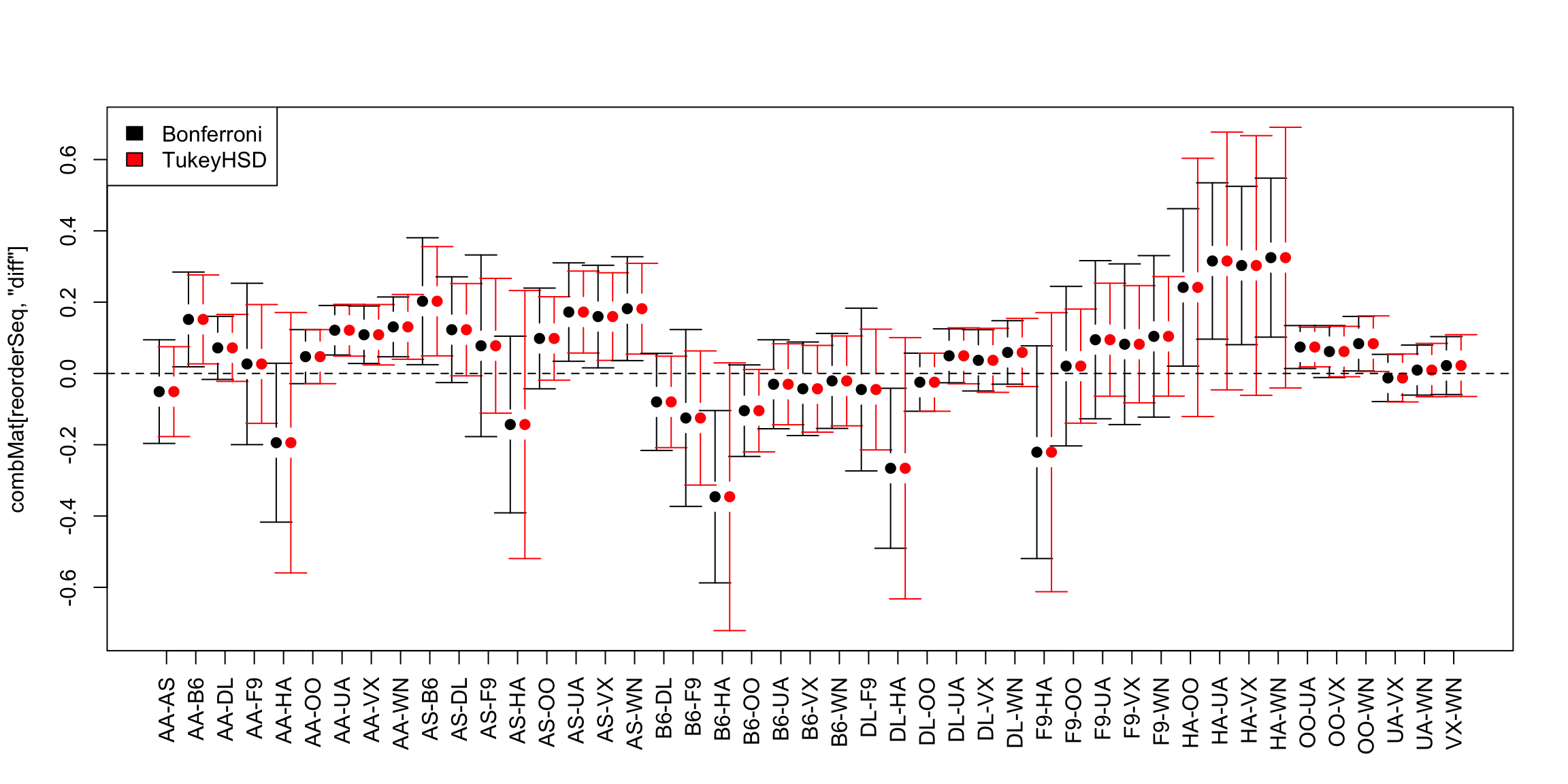
What differences do you see?
Which to use?
The TukeyHSD is a very specific correction – it is only valid for doing pairwise comparisons with the t-test. Bonferonni, on the other hand, can be used with any set of p-values from any test, e.g. permutation, and even if not all of the tests are pairwise comparisons.
In fact the distribution of \(X\) and \(|X|\) are related, and thus we can simplify our life by considering just \(|X|\).↩
Namely, if the data can be assumed to be exchangeable under the null hypothesis, then the permutation test is also a valid test.↩
\(X+Y \sim N(\mu_1+\mu_2, \sigma_1^2+\sigma_2^2+2cov(X,Y))\), where \(cov\) is the covariance between \(X\) and \(Y\)↩
And in fact, there are many variations of the CLT, which go beyond i.i.d samples↩
There are rare cases in comparing means where you might consider only evidence against the null that is positive (or negative). In this case you would then calculate the p-value correspondingly. These are called “one-sided” tests, for the same value of the observed statistic \(Z\) they give you smaller p-values, and they are usually only a good idea in very specific examples.↩
Indeed, the central limit theorem requires large data sizes, and how large a sample you need for the central limit theorem to give you a good approximation also depends on things about the distribution of the data, like how symmetric the distribution is.↩
In fact, if we were working with the difference in the means, rather than the t-statistics, which estimates the variance, the permutation test would give exactly the same answer since the log is a monotone transformation.↩
At least those tests based on the central limit theorem!↩
In fact, this is not an accurate statement because these tests are reusing the same data, so the data in each test are not independent, and the probabilities don’t work out like that. But it is reasonable for understanding the concepts here.↩
Indeed this true of all of science, which relies on hypothesis testing, so one always has to remember the importance of the iterative process of science to re-examine past experiments.↩
We can test a null hypothesis without having a specific parameter of interest that we are estimating. For example, the Chi-squared test that you may have seen in an introductory statistic class tests whether two discrete distributions are independent, but there is no single parameter that we are estimating.↩
There are many different strategies for calculating a bootstrap CI from the distribution of \(\hat{\delta}^*\); this method called the percentile method and is the most common and widespread. It doesn’t exactly correspond to the \(v_1\), \(v_2\) strategy from above – known as using a pivotal statistic. If it looks like the \(v_1\), \(v_2\) method is backward compared to the percentile method, it pretty much is! But both methods are legitimate methods for creating bootstrap intervals and we focus on the percentile method because of it’s simplicity and wider applicability.↩
There are methods for accounting for a small amount of bias with the bootstrap, but if the statistic is wildly biased away from the truth, then the bootstrap will not work.↩
This clearly assumes what is a “reasonable” definition of "close’’ between distributions that we won’t go into right now.↩
If it looks like this method is backward compared to the percentile method, it pretty much is! But both methods are legitimate methods for creating bootstrap intervals.↩
From https://statisticsbyjim.com/hypothesis-testing/confidence-intervals-compare-means/↩