Chapter 6 Multiple Regression
## Linking to ImageMagick 6.9.12.3
## Enabled features: cairo, fontconfig, freetype, heic, lcms, pango, raw, rsvg, webp
## Disabled features: fftw, ghostscript, x11
This chapter deals with the regression problem where the goal is to understand the relationship between a specific variable called the response or dependent variable (\(y\)) and several other related variables called explanatory or independent variables or more generally covariates. This is an extension of our previous discussion of simple regression, where we only had a single covariate (\(x\)).
6.1 Examples
We will go through some specific examples to demonstrate the range of the types of problems we might consider in this chapter.
- Prospective buyers and sellers might want to understand how the price of a house depends on various characteristics of the house such as the total above ground living space, total basement square footage, lot area, number of cars that can be parked in the garage, construction year and presence or absence of a fireplace. This is an instance of a regression problem where the response variable is the house price and the other characteristics of the house listed above are the explanatory variables.
This dataset contains information on sales of houses in Ames, Iowa from 2006 to 2010. The full dataset can be obtained by following links given in the paper: (https://ww2.amstat.org/publications/jse/v19n3/decock.pdf)). I have shortened the dataset slightly to make life easier for us.
dataDir <- "../finalDataSets"
dd = read.csv(file.path(dataDir, "Ames_Short.csv"),
    header = T, stringsAsFactors = TRUE)
pairs(dd)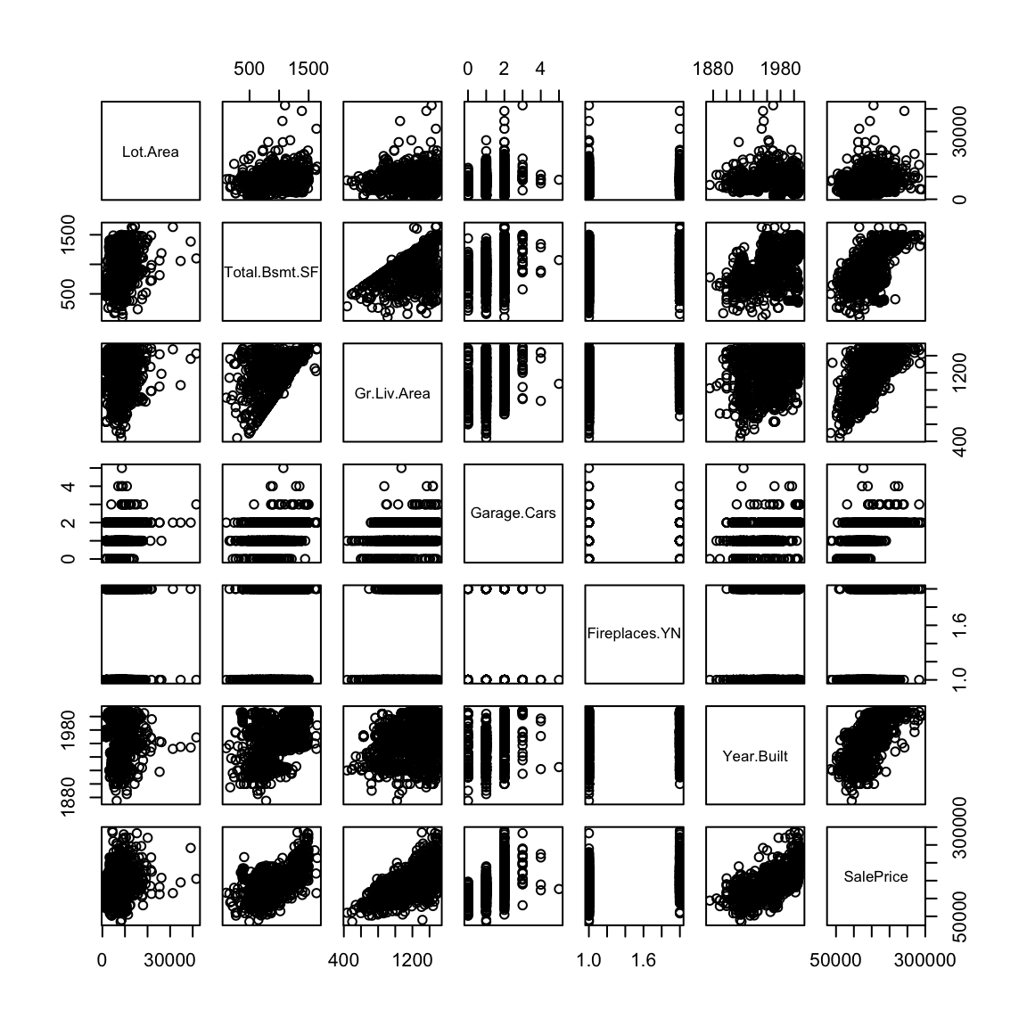
- A bike rental company wants to understand how the number of bike rentals in a given hour depends on environmental and seasonal variables (such as temperature, humidity, presence of rain etc.) and various other factors such as weekend or weekday, holiday etc. This is also an instance of a regression problems where the response variable is the number of bike rentals and all other variables mentioned are explanatory variables.
bike <- read.csv(file.path(dataDir, "DailyBikeSharingDataset.csv"),
    stringsAsFactors = TRUE)
bike$yr <- factor(bike$yr)
bike$mnth <- factor(bike$mnth)
pairs(bike[, 11:16])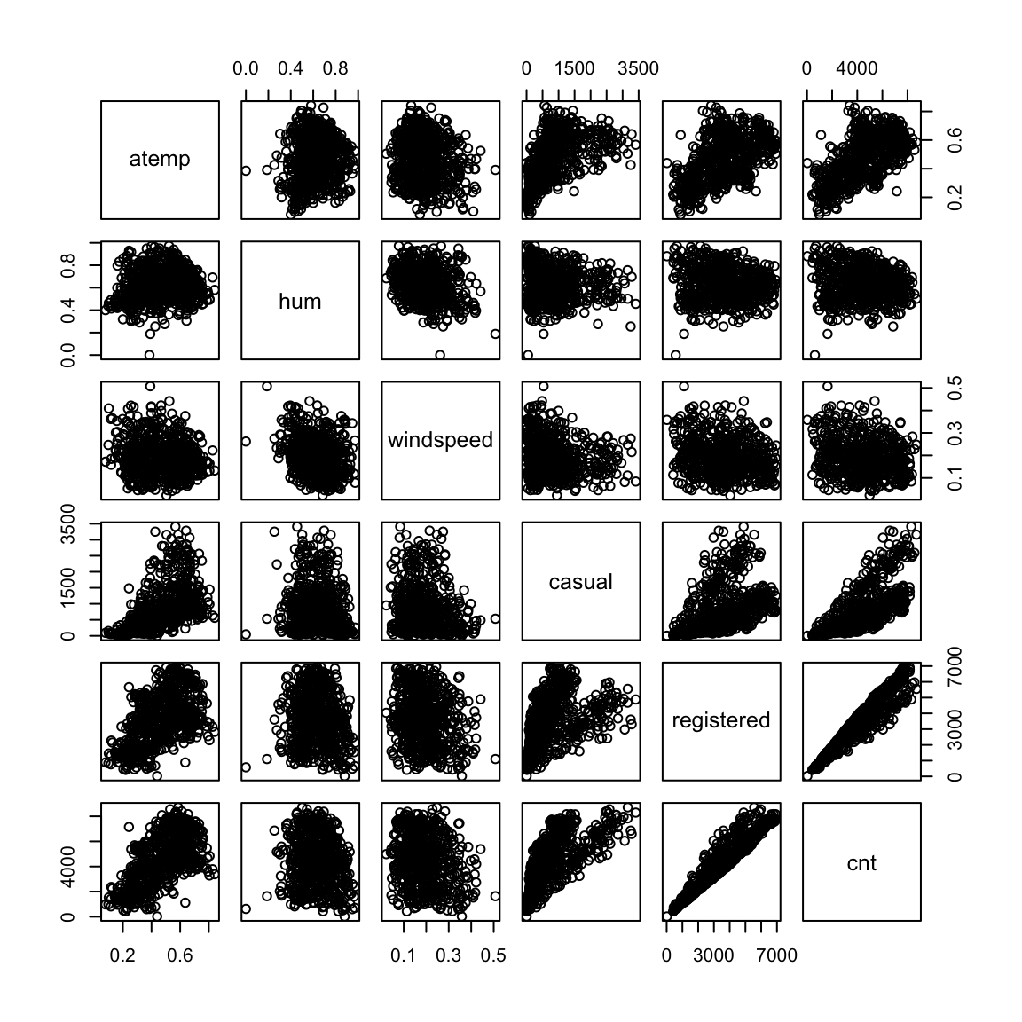
We might want to understand how the retention rates of colleges depend on various aspects such as tuition fees, faculty salaries, number of faculty members that are full time, number of undergraduates enrolled, number of students on federal loans etc. using our college data from before. This is again a regression problem with the response variable being the retention rate and other variables being the explanatory variables.
We might be interested in understanding the proportion of my body weight that is fat (body fat percentage). Directly measuring this quantity is probably hard but I can easily obtain various body measurements such as height, weight, age, chest circumeference, abdomen circumference, hip circumference and thigh circumference. Can we predict my body fat percentage based on these measurements? This is again a regression problem with the response variable being body fat percentage and all the measurements are explanatory variables.
Body fat percentage (computed by a complicated underwater weighing technique) along with various body measurements are given for 252 adult men.
body = read.csv(file.path(dataDir, "bodyfat_short.csv"),
    header = T, stringsAsFactors = TRUE)
pairs(body)
There are outliers in the data and they make it hard to look at the relationships between the variables. We can try to look at the pairs plots after deleting some outlying observations.
ou1 = which(body$HEIGHT < 30)
ou2 = which(body$WEIGHT > 300)
ou3 = which(body$HIP > 120)
ou = c(ou1, ou2, ou3)
pairs(body[-ou, ])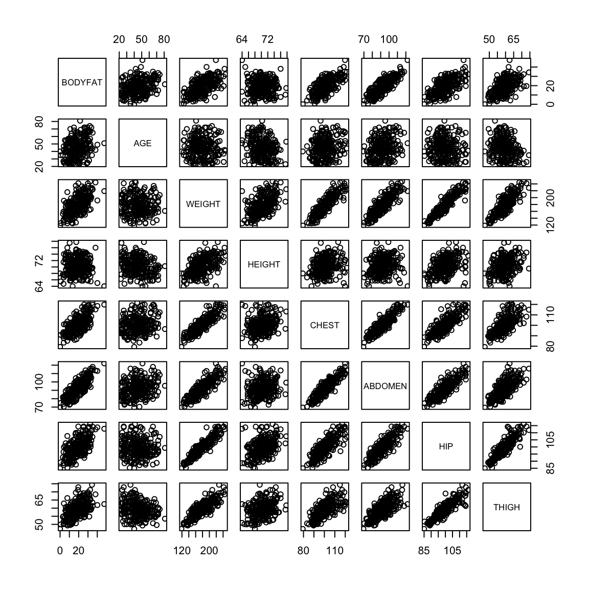
6.2 The nature of the `relationship’
Notice that in these examples, the goals of the analysis shift depending on the example from truly wanting to just be able to predict future observations (e.g. body-fat), wanting to have insight into how to the variables are related to the response (e.g. college data), and a combination of the two (e.g. housing prices and bike sharing).
What do we mean by the relationship of a explanatory variable to a response? There are multiple valid interpretations that are used in regression that are important to distinguish.
- The explanatory variable is a good predictor of the response.
The explanatory variable is necessary for good prediction of the response (among the set of variables we are considering).
Changes in the explanatory variable cause the response to change (causality).
We can visualize the difference in the first and second with plots. Being a good predictor is like the pairwise scatter plots from before, in which case both thigh and abdominal circumference are good predictors of percentage of body fat.
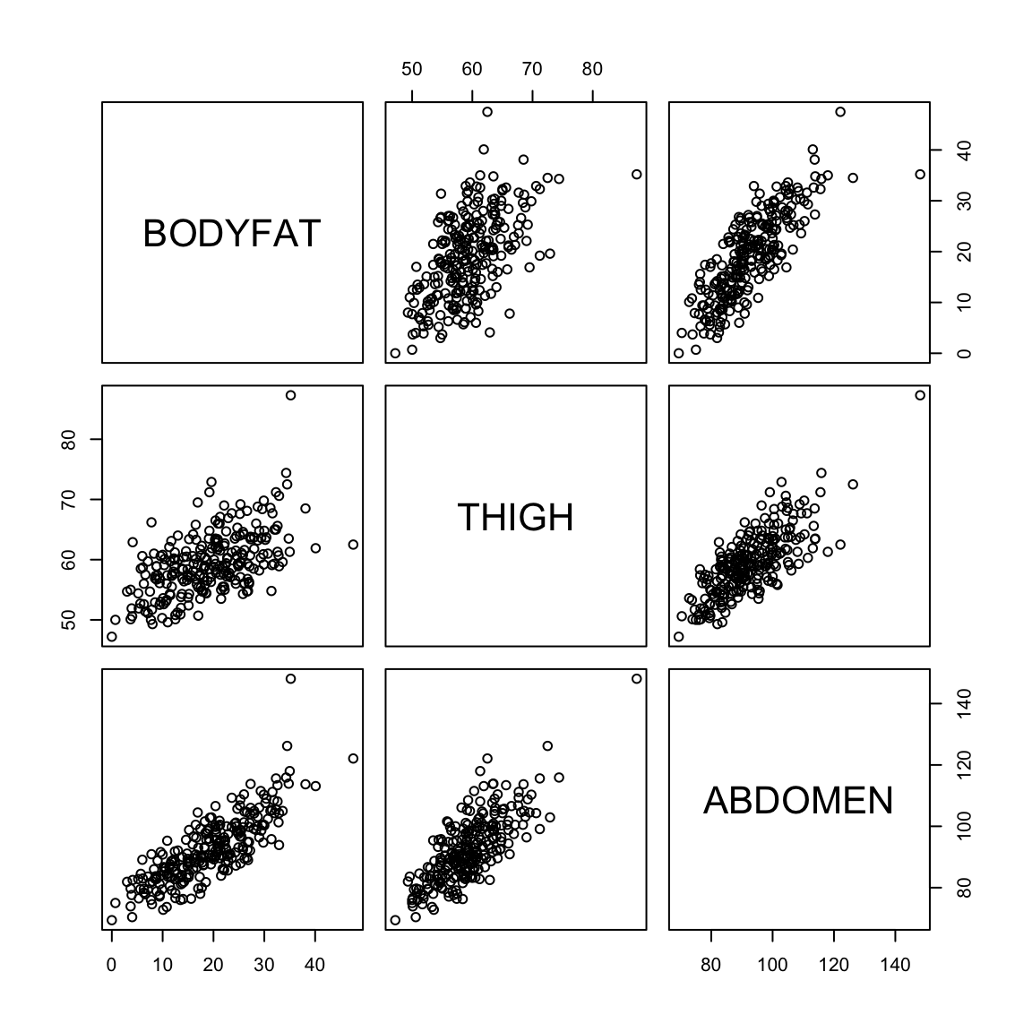
But in fact if we know the abdominal circumference, the thigh circumference does not tell us much more. A coplot visualizes this relationship, by plotting the relationship between two variables, conditional on the value of another. In otherwords, it plots the scatter plot of percent body fat against thigh, but only for those points for abdomen in a certain range (with the ranges indicated at the top).
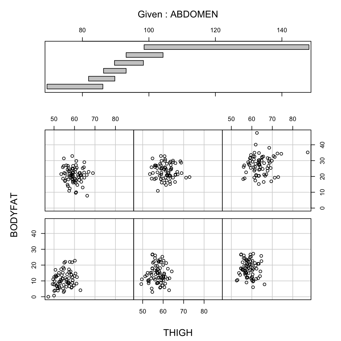
We see there is no longer a strong relationship between percentage body fat and thigh circumference for specific values of abdomen circumference
The same is not true, however, for the reverse,
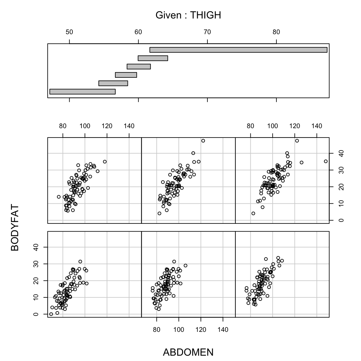
We will see later in the course when we have many variables the answers to these three questions are not always the same (and that we can’t always answer all of them). We will almost always be able to say something about the first two, but the last is often not possible.
6.2.1 Causality
Often a (unspoken) goal of linear regression can be to determine whether something `caused’ something else. It is critical to remember that whether you can attribute causality to a variable depends on how your data was collected. Specifically, most people often have observational data, i.e. they sample subjects or units from the population and then measure the variables that naturally occur on the units they happen to sample. In general, you cannot determine causality by just collecting observations on existing subjects. You can only observe what is likely to naturally occur jointly in your population, often due to other causes. Consider the following data on the relationship between the murder rate and the life expectancy of different states or that of Illiteracy and Frost:
st <- as.data.frame(state.x77)
colnames(st)[4] = "Life.Exp"
colnames(st)[6] = "HS.Grad"
par(mfrow = c(1, 2))
with(st, plot(Murder, Life.Exp))
with(st, plot(Frost, Illiteracy))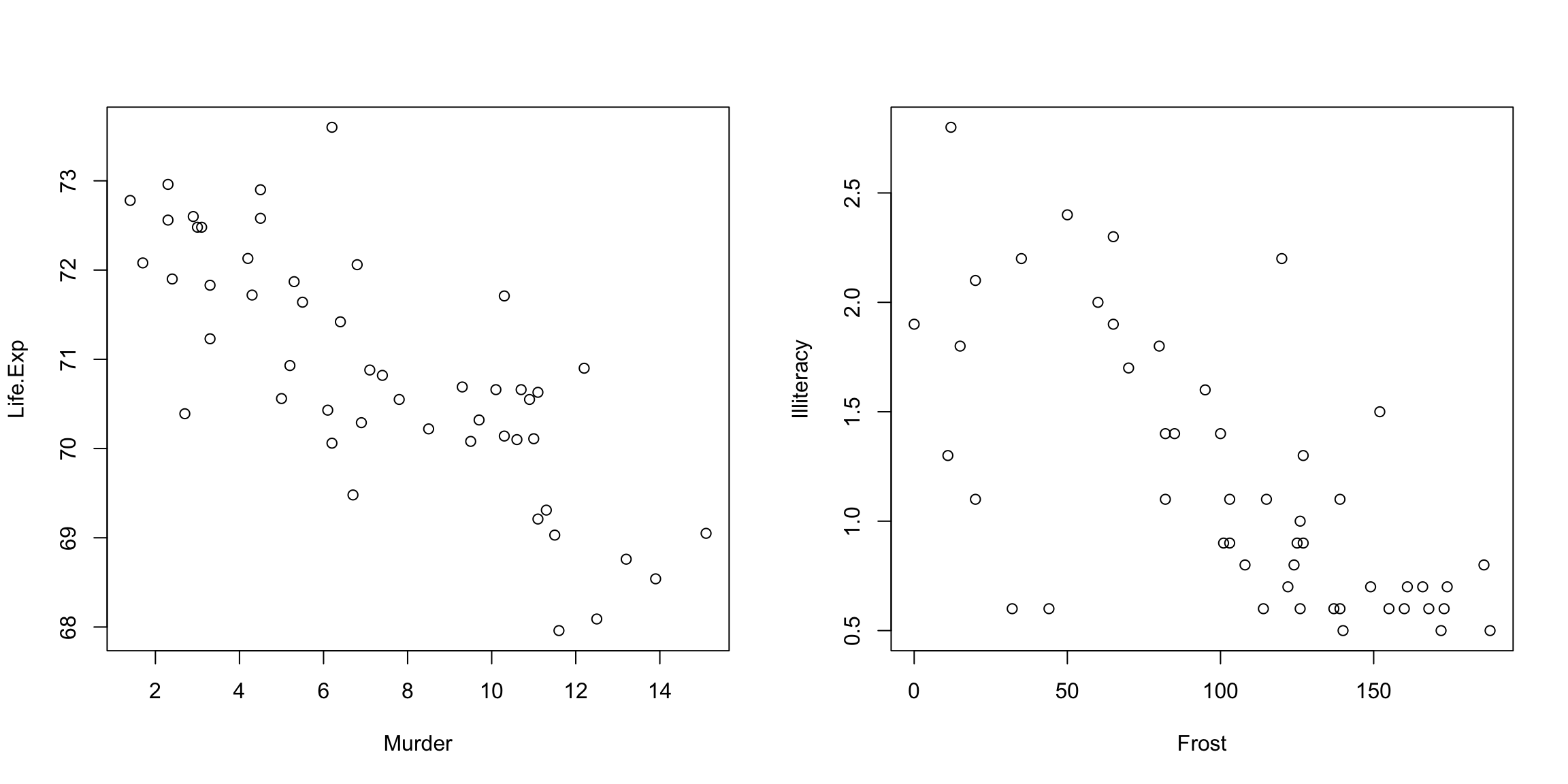
What do you observe in the plotted relationship between the murder rate and the life expectancy ? What about between frost levels and illiteracy? What would it mean to (wrongly) assume causality here?
It is a common mistake in regression to to jump to the conclusion that one variable causes the other, but all you can really say is that there is a strong relationship in the population, i.e. when you observe one value of the variable you are highly likely to observed a particular value of the other.
Can you ever claim causality? Yes, if you run an experiment; this is where you assign what the value of the predictors are for every observation independently from any other variable. An example is a clinical trial, where patients are randomly assigned a treatment.
It’s often not possible to run an experiment, especially in the social sciences or working with humans (you can’t assign a murder rate in a state and sit back and see what the effect is on life expectancy!). In the absence of an experiment, it is common to collect a lot of other variables that might also explain the response, and ask our second question – “how necessary is it (in addition to these other variables)?” with the idea that this is a proxy for causality. This is sometime called “controlling” for the effect of the other variables, but it is important to remember that this is not the same as causality.
Regardless, the analysis of observational and experimental data often both use linear regression.53 It’s what conclusions you can draw that differ.
6.3 Multiple Linear Regression
The body fat dataset is a useful one to use to explain linear regression because all of the variables are continuous and the relationships are reasonably linear.
Let us look at the plots between the response variable (bodyfat) and all the explanatory variables (we’ll remove the outliers for this plot).
par(mfrow = c(3, 3))
for (i in 2:8) {
    plot(body[-ou, i], body[-ou, 1], xlab = names(body)[i],
        ylab = "BODYFAT")
}
par(mfrow = c(1, 1))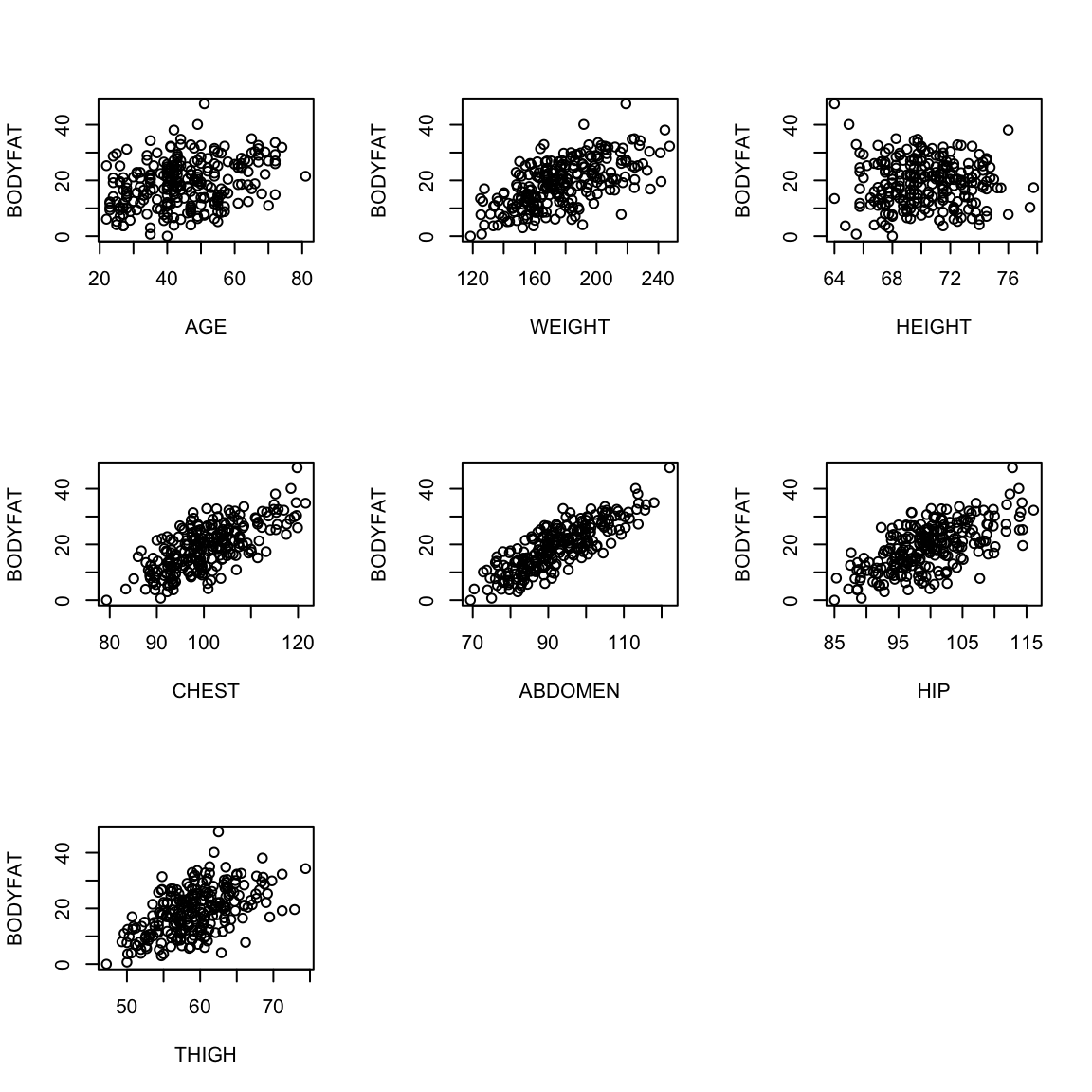
Most pairwise relationships seem to be linear. The clearest relationship is between bodyfat and abdomen. The next clearest is between bodyfat and chest.
We can expand the simple regression we used earlier to include more variables. \[y=\beta_0+\beta_1 x^{(1)}+\beta_2 x^{(2)}+\ldots \]
6.3.1 Regression Line vs Regression Plane
In simple linear regression (when there is only one explanatory variable), the fitted regression equation describes a line. If we have two variables, it defines a plane. This plane can be plotted in a 3D plot when there are two explanatory variables. When the number of explanatory variables is 3 or more, we have a general linear combination54 and we cannot plot this relationship.
To illustrate this, let us fit a regression equation to bodyfat percentage in terms of age and chest circumference:
We can visualize this 3D plot:
library(scatterplot3d)
sp = scatterplot3d(body$AGE, body$CHEST, body$BODYFAT)
sp$plane3d(ft2, lty.box = "solid", draw_lines = TRUE,
    draw_polygon = TRUE, col = "red")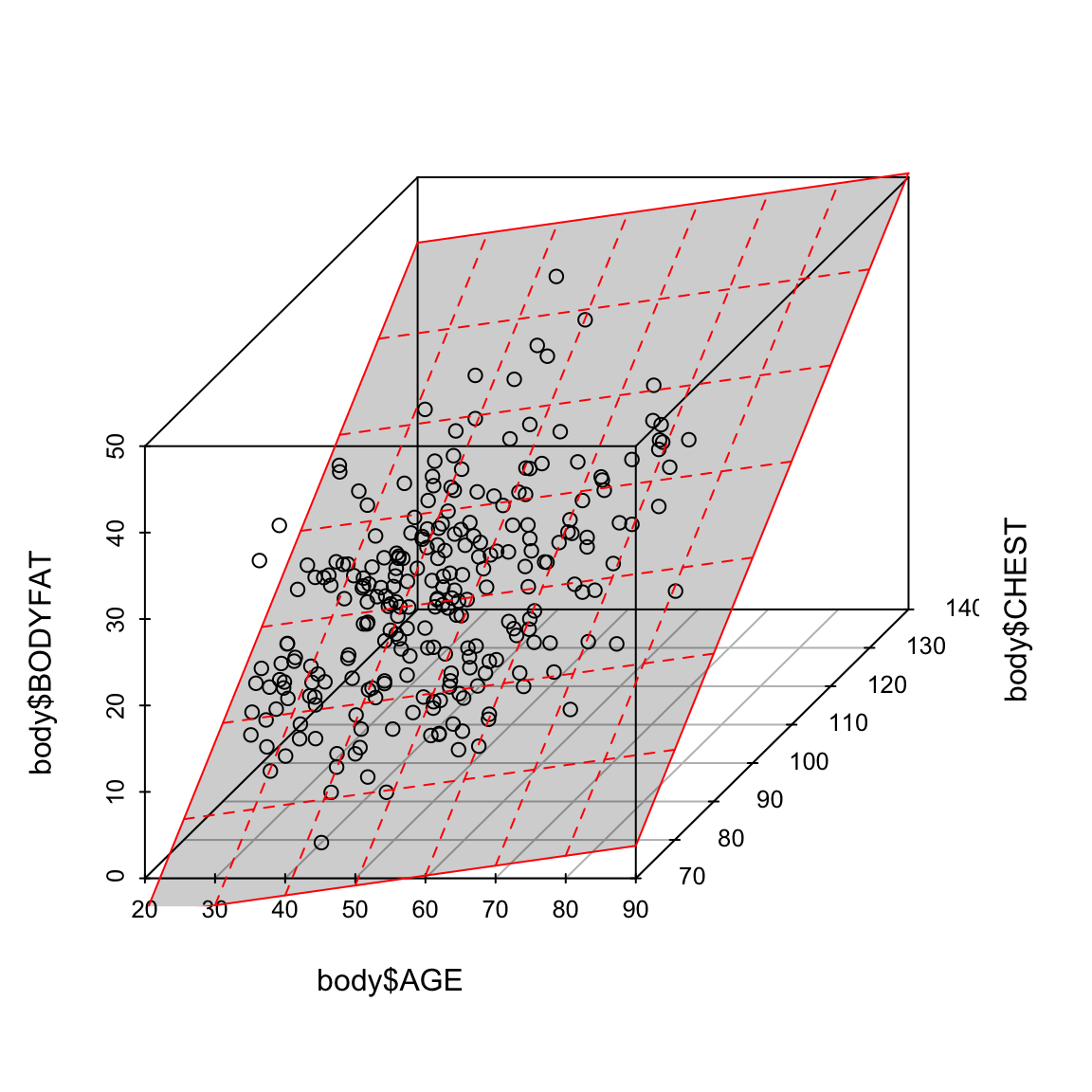
6.3.2 How to estimate the coefficients?
We can use the same principle as before. Specifically, for any selection of our \(\beta_j\) coefficients, we get a predicted or fitted value \(\hat{y}\). Then we can look for the \(\beta_j\) which minimize our loss \[\sum_{i=1}^n \ell(y_i,\hat{y}_i)\] Again, standard regression uses squared-error loss, \[\sum_{i=1}^n (y_i-\hat{y}_i)^2.\]
We again can fit this by using lm in R, with similar syntax as before:
##
## Call:
## lm(formula = BODYFAT ~ AGE + WEIGHT + HEIGHT + CHEST + ABDOMEN +
##     HIP + THIGH, data = body)
##
## Residuals:
##      Min       1Q   Median       3Q      Max
## -11.0729  -3.2387  -0.0782   3.0623  10.3611
##
## Coefficients:
##               Estimate Std. Error t value Pr(>|t|)
## (Intercept) -3.748e+01  1.449e+01  -2.585  0.01031 *
## AGE          1.202e-02  2.934e-02   0.410  0.68246
## WEIGHT      -1.392e-01  4.509e-02  -3.087  0.00225 **
## HEIGHT      -1.028e-01  9.787e-02  -1.051  0.29438
## CHEST       -8.312e-04  9.989e-02  -0.008  0.99337
## ABDOMEN      9.685e-01  8.531e-02  11.352  < 2e-16 ***
## HIP         -1.834e-01  1.448e-01  -1.267  0.20648
## THIGH        2.857e-01  1.362e-01   2.098  0.03693 *
## ---
## Signif. codes:  0 '***' 0.001 '**' 0.01 '*' 0.05 '.' 0.1 ' ' 1
##
## Residual standard error: 4.438 on 244 degrees of freedom
## Multiple R-squared:  0.7266, Adjusted R-squared:  0.7187
## F-statistic: 92.62 on 7 and 244 DF,  p-value: < 2.2e-16
In fact, if we want to use all the variables in a data.frame we can use a simpler notation:
Notice how similar the output to the function above is to the case of simple linear regression. R has fit a linear equation for the variable BODYFAT in terms of the variables AGE, WEIGHT, HEIGHT, CHEST, ABDOMEN, HIP and THIGH. Again, the summary of the output gives each variable and its estimated coefficient,
\[\begin{align*} BODYFAT &= -37.48 + 0.012*AGE - 0.139*WEIGHT - 0.102*HEIGHT \\ & - 0.0008*CHEST + 0.968*ABDOMEN - 0.183*HIP + 0.286*THIGH \nonumber \end{align*}\]
We can also write down explicit equations for the estimates of the \(\hat{\beta}_j\) when we use squared-error loss, though we won’t give them here (they are usually given in matrix notation).
6.3.3 Interpretation of the regression equation
Here the coefficient \(\hat{\beta}_1\) is interpreted as the average increase in \(y\) for unit increase in \(x^{(1)}\), provided all other explanatory variables \(x^{(2)}, \dots, x^{(p)}\) are kept constant. More generally for \(j \geq 1\), the coefficient \(\hat{\beta}_j\) is interpreted as the average increase in \(y\) for unit increase in \(x^{(j)}\) provided all other explanatory variables \(x^{(k)}\) for \(k \neq j\) are kept constant. The intercept \(\hat{\beta}_0\) is interpreted as the average value of \(y\) when all the explanatory variables are equal to zero.
In the body fat example, the fitted regression equation as we have seen is: \[\begin{align*} BODYFAT &= -37.48 + 0.012*AGE - 0.139*WEIGHT - 0.102*HEIGHT \\ & - 0.0008*CHEST + 0.968*ABDOMEN - 0.183*HIP + 0.286*THIGH \end{align*}\] The coefficient of \(0.968\) can be interpreted as the average percentage increase in bodyfat percentage per unit (i.e., \(1\) cm) increase in Abdomen circumference provided all the other explanatory variables age, weight, height, chest circumference, hip circumference and thigh circumference are kept unchanged.
Do the signs of the fitted regression coefficients make sense?
6.3.3.1 Scaling and the size of the coefficient
It’s often tempting to look at the size of the \(\beta_j\) as a measure of how “important” the variable \(j\) is in predicting the response \(y\). However, it’s important to remember that \(\beta_j\) is relative to the scale of the input \(x^{(j)}\) – it is the change in \(y\) for one unit change in \(x^{(j)}\). So, for example, if we change from measurements in cm to mm (i.e. multiply \(x^{(j)}\) by 10) then we will get a \(\hat{\beta}_j\) that is divided by 10:
tempBody <- body
tempBody$ABDOMEN <- tempBody$ABDOMEN * 10
ftScale = lm(BODYFAT ~ ., data = tempBody)
cat("Coefficients with Abdomen in mm:\n")
## Coefficients with Abdomen in mm:## (Intercept) AGE WEIGHT HEIGHT CHEST
## -3.747573e+01 1.201695e-02 -1.392006e-01 -1.028485e-01 -8.311678e-04
## ABDOMEN HIP THIGH
## 9.684620e-02 -1.833599e-01 2.857227e-01## Coefficients with Abdomen in cm:## (Intercept) AGE WEIGHT HEIGHT CHEST
## -3.747573e+01 1.201695e-02 -1.392006e-01 -1.028485e-01 -8.311678e-04
## ABDOMEN HIP THIGH
## 9.684620e-01 -1.833599e-01 2.857227e-01For this reason, it is not uncommon to scale the explanatory variables – i.e. divide each variable by its standard deviation – before running the regression:
tempBody <- body
tempBody[, -1] <- scale(tempBody[, -1])
ftScale = lm(BODYFAT ~ ., data = tempBody)
cat("Coefficients with variables scaled:\n")
## Coefficients with variables scaled:## (Intercept) AGE WEIGHT HEIGHT CHEST ABDOMEN
## 19.15079365 0.15143812 -4.09098792 -0.37671913 -0.00700714 10.44300051
## HIP THIGH
## -1.31360120 1.50003073## Coefficients on original scale:## (Intercept) AGE WEIGHT HEIGHT CHEST
## -3.747573e+01 1.201695e-02 -1.392006e-01 -1.028485e-01 -8.311678e-04
## ABDOMEN HIP THIGH
## 9.684620e-01 -1.833599e-01 2.857227e-01## Sd per variable:## AGE WEIGHT HEIGHT CHEST ABDOMEN HIP THIGH
## 12.602040 29.389160 3.662856 8.430476 10.783077 7.164058 5.249952## Ratio of scaled lm coefficient to original lm coefficient## AGE WEIGHT HEIGHT CHEST ABDOMEN HIP THIGH
## 12.602040 29.389160 3.662856 8.430476 10.783077 7.164058 5.249952Now the interpretation of the \(\beta_j\) is that per standard deviation change in the variable \(x^{j}\), what is the change in \(y\), again all other variables remaining constant.
6.3.3.2 Correlated Variables
The interpretation of the coefficient \(\hat{\beta}_j\) depends crucially on the other explanatory variables \(x^{(k)}, k \neq j\) that are present in the equation (this is because of the phrase “all other explanatory variables kept constant”).
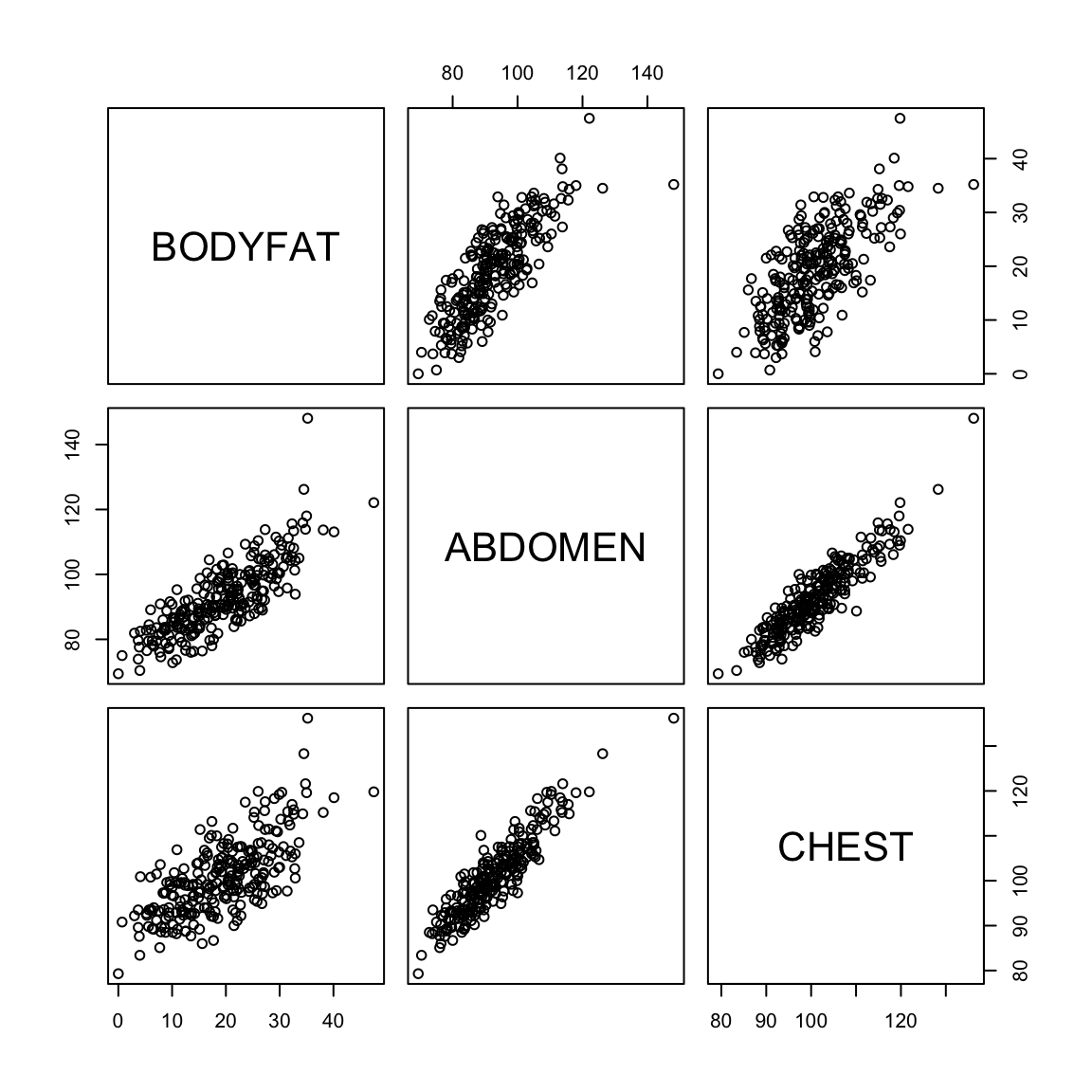
For the bodyfat data, we have seen that the variables chest thigh and hip and abdomen circumference are highly correlated:
##               HIP     THIGH   ABDOMEN     CHEST
## HIP     1.0000000 0.8964098 0.8740662 0.8294199
## THIGH   0.8964098 1.0000000 0.7666239 0.7298586
## ABDOMEN 0.8740662 0.7666239 1.0000000 0.9158277
## CHEST   0.8294199 0.7298586 0.9158277 1.0000000
Notice that both CHEST and ABDOMEN are linearly related to BODYFAT
Individual linear regressions would show very significant values for both CHEST and ABDOMEN:
##                Estimate Std. Error   t value     Pr(>|t|)
## (Intercept) -51.1715853 4.51985295 -11.32152 2.916303e-24
## CHEST 0.6974752 0.04467377 15.61263 8.085369e-39## Estimate Std. Error t value Pr(>|t|)
## (Intercept) -39.2801847 2.66033696 -14.76512 6.717944e-36
## ABDOMEN 0.6313044 0.02855067 22.11172 9.090067e-61But when we look at the multiple regression, we see ABDOMEN is significant and not CHEST:
##             Estimate Std. Error t value Pr(>|t|)
## (Intercept)  -37.476     14.495  -2.585    0.010
## AGE            0.012      0.029   0.410    0.682
## WEIGHT        -0.139      0.045  -3.087    0.002
## HEIGHT        -0.103      0.098  -1.051    0.294
## CHEST         -0.001      0.100  -0.008    0.993
## ABDOMEN        0.968      0.085  11.352    0.000
## HIP           -0.183      0.145  -1.267    0.206
## THIGH          0.286      0.136   2.098    0.037
This is because coefficient assigned to ABDOMEN and CHEST tells us how the response changes as the other variables stay the same. This interpretation of \(\beta_j\) ties directly back to our coplots and can help us understand how this is different from an individual regression on each variable. A coplot plots the response (BODYFAT) against a variable for a “fixed” value of another variable (i.e. a small range of values). When we do this with ABDOMEN for fixed values of CHEST we still see a strong relationship between ABDOMEN and BODYFAT
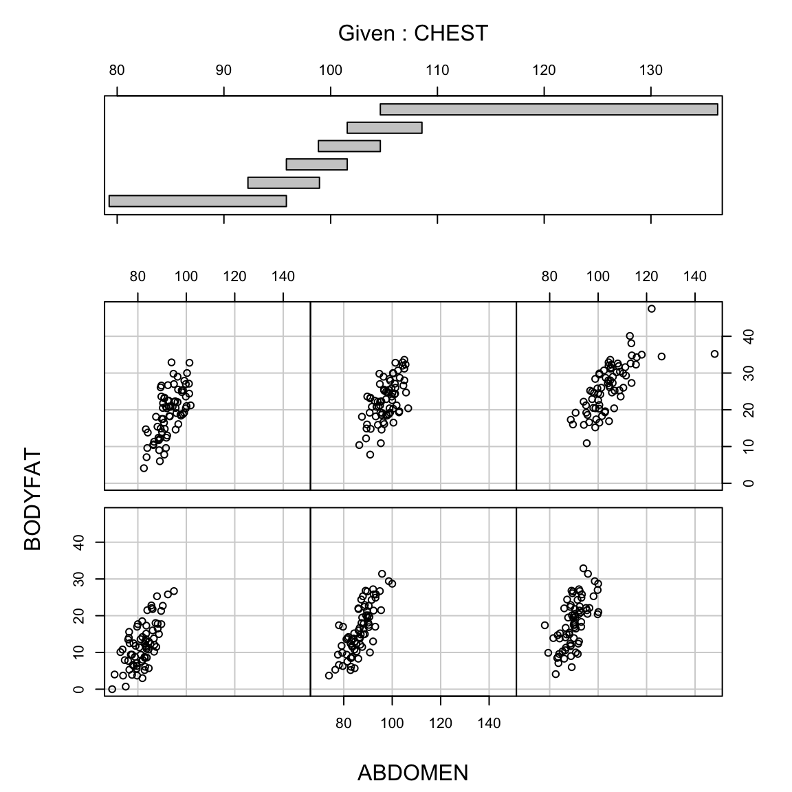
But the other way around shows us for a “fixed” value of ABDOMEN, CHEST doesn’t have much relationship with BODYFAT
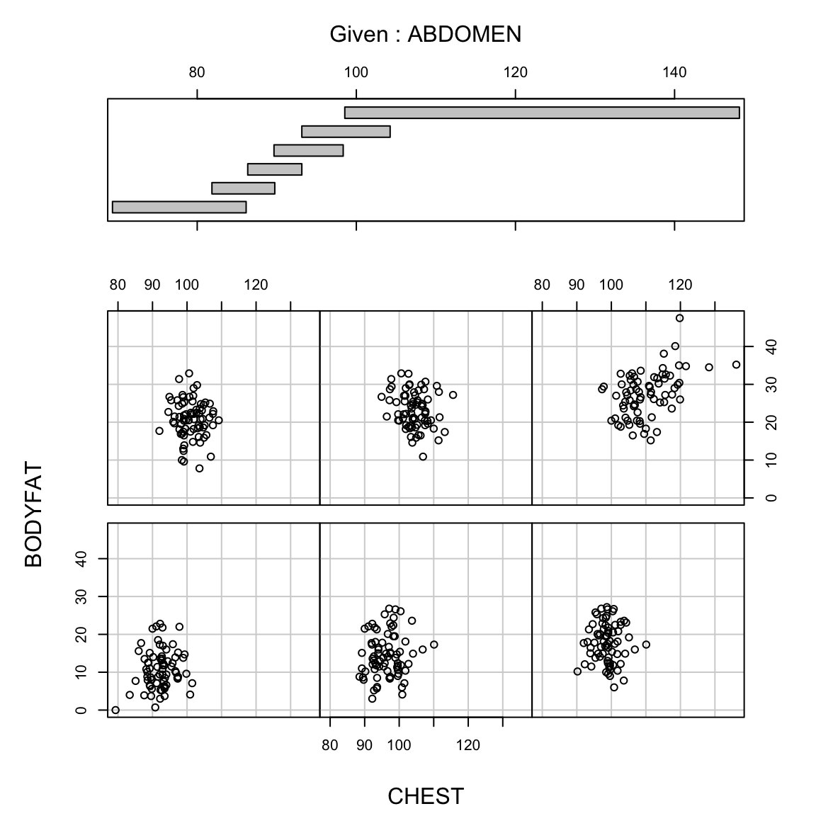
This is the basic idea behind the interpretation of the coefficient \(\beta_j\) in a multiple regression, only for regression it is holding all of the other variables fixed, not just one.
What if we didn’t include ABDOMEN and THIGH in our regression? (ie. a model based on age, weight, height, chest and hip):
## (Intercept)         AGE      WEIGHT      HEIGHT       CHEST     ABDOMEN
##    -37.4757      0.0120     -0.1392     -0.1028     -0.0008      0.9685
##         HIP       THIGH
## -0.1834 0.2857## (Intercept) AGE WEIGHT HEIGHT CHEST HIP
## -53.9871 0.1290 -0.0526 -0.3146 0.5148 0.4697See now that the actually coefficient values are quite different from the
previous one – and they have
different interpretations as well. In this model, CHEST is now very significant.
##             Estimate Std. Error t value Pr(>|t|)
## (Intercept) -53.9871    17.1362 -3.1505   0.0018
## AGE           0.1290     0.0308  4.1901   0.0000
## WEIGHT       -0.0526     0.0534 -0.9841   0.3260
## HEIGHT       -0.3146     0.1176 -2.6743   0.0080
## CHEST         0.5148     0.1080  4.7662   0.0000
## HIP           0.4697     0.1604  2.9286   0.0037
It’s important to remember that the \(\beta_j\) are not a fixed, immutable property of the variable, but are only interpretable in the context of the other variables. So the interpretation of \(\hat{\beta}_j\) (and it’s significance) is a function of the \(x\) data you have. If you only observe \(x^{j}\) large when \(x^{(k)}\) is also large (i.e. strong and large positive correlation), then you have little data where \(x^{(j)}\) is changing over a range of values while \(x^{(k)}\) is basically constant. For example, if you fix ABDOMEN to be 100in, the range of values of CHEST is tightly constrained to roughly 95-112in, i.e. CHEST doesn’t actually change much in the population if you fix ABDOMEN.
Here’s some simulated data demonstrating this. Notice both variables are pretty correlated with the response \(y\)
set.seed(275382)
n <- 300
trueQuality <- rnorm(n)
score2 <- (trueQuality + 100) * 0.5 + rnorm(n, sd = 0.1)
score1 <- (trueQuality + 80) * 0.5 + rnorm(n, sd = 0.1)
y <- 8 + 10 * score1 + 10 * score2 + rnorm(n, sd = 15)
x <- data.frame(y, score1, score2)
pairs(x)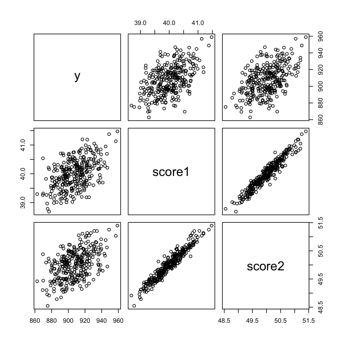
But if I look at the regression summary, I don’t get any significance.
##
## Call:
## lm(formula = y ~ ., data = x)
##
## Residuals:
##     Min      1Q  Median      3Q     Max
## -46.067 -10.909   0.208   9.918  38.138
##
## Coefficients:
##             Estimate Std. Error t value Pr(>|t|)
## (Intercept)  110.246     97.344   1.133    0.258
## score1         8.543      6.301   1.356    0.176
## score2         9.113      6.225   1.464    0.144
##
## Residual standard error: 15.09 on 297 degrees of freedom
## Multiple R-squared:  0.2607, Adjusted R-squared:  0.2557
## F-statistic: 52.37 on 2 and 297 DF,  p-value: < 2.2e-16
However, individually, each score is highly significant in predicting \(y\)
##
## Call:
## lm(formula = y ~ score1, data = x)
##
## Residuals:
##     Min      1Q  Median      3Q     Max
## -47.462 -10.471   0.189  10.378  38.868
##
## Coefficients:
##             Estimate Std. Error t value Pr(>|t|)
## (Intercept)  211.072     68.916   3.063  0.00239 **
## score1        17.416      1.723  10.109  < 2e-16 ***
## ---
## Signif. codes:  0 '***' 0.001 '**' 0.01 '*' 0.05 '.' 0.1 ' ' 1
##
## Residual standard error: 15.12 on 298 degrees of freedom
## Multiple R-squared:  0.2554, Adjusted R-squared:  0.2529
## F-statistic: 102.2 on 1 and 298 DF, p-value: < 2.2e-16##
## Call:
## lm(formula = y ~ score2, data = x)
##
## Residuals:
## Min 1Q Median 3Q Max
## -44.483 -11.339 0.195 11.060 40.327
##
## Coefficients:
## Estimate Std. Error t value Pr(>|t|)
## (Intercept) 45.844 85.090 0.539 0.59
## score2 17.234 1.701 10.130 <2e-16 ***
## ---
## Signif. codes: 0 '***' 0.001 '**' 0.01 '*' 0.05 '.' 0.1 ' ' 1
##
## Residual standard error: 15.11 on 298 degrees of freedom
## Multiple R-squared: 0.2561, Adjusted R-squared: 0.2536
## F-statistic: 102.6 on 1 and 298 DF, p-value: < 2.2e-16They just don’t add further information when added to the existing variable already included. Looking at the coplot, we can visualize this – for each bin of score 2 (i.e. as close as we can get to constant), we have very little further change in \(y\).
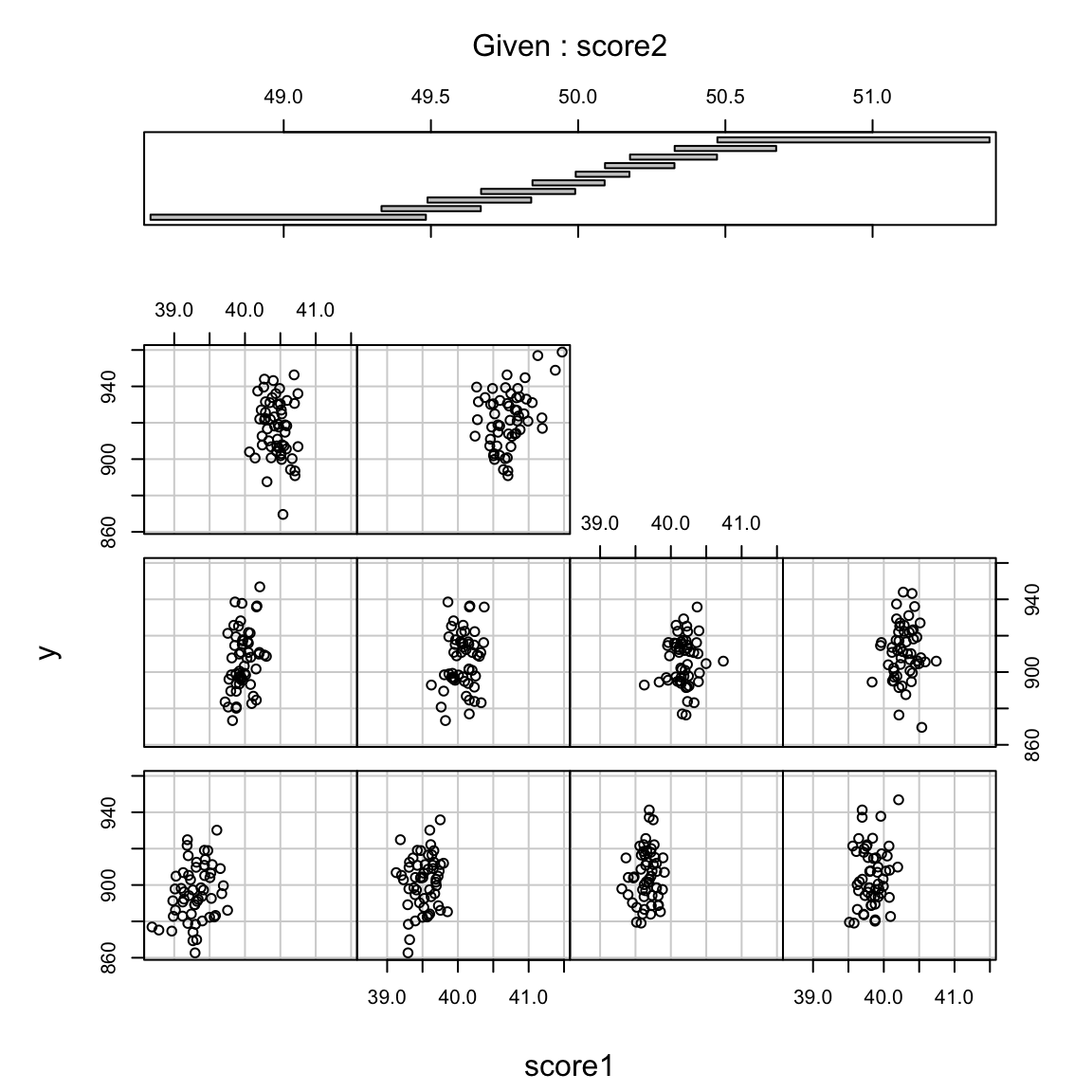
We will continually return the effect of correlation in understanding multiple regression.
What kind of relationship with \(y\) does \(\beta_j\) measure?
If we go back to our possible questions we could ask about the relationship between a single variable \(j\) and the response, then \(\hat{\beta}_j\) answers the second question: how necessary is variable \(j\) to the predition of \(y\) above and beyond the other variables? We can see this in our above description of “being held constant” – if when the other variables aren’t changing, \(\hat{\beta}_j\) tells us how much \(y\) moves on average as only \(x^{(j)}\) changes. If \(\hat{\beta}_j\) is close to \(0\), then changes in \(x^{(j)}\) aren’t affecting \(y\) much for fixed values of the other coordinates.
Why the \(\beta_j\) does not measure causality
Correlation in our variables is one important reason why the value of \(\beta_j\) does not measure causality, i.e whether a change in \(x^{(j)}\) caused \(y\) to change. If \(x^{(j)}\) is always large when \(x^{(k)}\) is large, there is no (or little) data to evaluate whether a large \(x^{(j)}\) in the presence of a small \(x^{(k)}\) would result in a large \(y\). 55
Again, it can be helpful to compare what you would expect if you could create a randomized experiment. You would choose individuals with a particular value of ABDOMEN circumference, say 100cm. Then for some individuals you would change their CHEST size to be 80cm and for others 120cm, and then measure the resulting BODYFAT. Just writing it down makes it clear why such an experiment is impossible – and also why circumference on its own is a poor candidate for causing anything. Rather internal bodily mechanisms result in all three variables (ABDOMEN, CHEST, and BODYFAT) to be larger, without one causing another.
6.4 Important measurements of the regression estimate
6.4.1 Fitted Values and Multiple \(R^2\)
Any regression equation can be used to predict the value of the
response variable given values of the explanatory variables, which we call \(\hat{y}(x)\). We can get a fitted value for any value \(x\). For
example, consider our original fitted regression equation obtained by applying
lm with bodyfat percentage against all of the variables as explanatory variables:
\[\begin{align*}
BODYFAT &= -37.48 + 0.01202*AGE - 0.1392*WEIGHT - 0.1028*HEIGHT \\
& - 0.0008312*CHEST + 0.9685*ABDOMEN - 0.1834*HIP + 0.2857*THIGH
\end{align*}\]
Suppose a person X (who is of 30 years of age, weighs 180 pounds and
is 70 inches tall) wants to find out his bodyfat percentage. Let us
say that he is able to measure his chest circumference as 90 cm,
abdomen circumference as 86 cm, hip circumference as 97 cm and thigh
circumference as 60 cm. Then he can simply use the regression equation
to predict his bodyfat percentage as:
bf.pred = -37.48 + 0.01202 * 30 - 0.1392 * 180 - 0.1028 *
    70 - 0.0008312 * 90 + 0.9685 * 86 - 0.1834 * 97 +
    0.2857 * 60
bf.pred
## [1] 13.19699The predictions given by the fitted regression equation *for each of the observations} are known as fitted values, \(\hat{y}_i=\hat{y}(x_i)\). For example, in the bodyfat dataset, the first observation (first row) is given by:
##   BODYFAT AGE WEIGHT HEIGHT CHEST ABDOMEN  HIP THIGH
## 1    12.3  23 154.25  67.75  93.1    85.2 94.5    59
The observed value of the response (bodyfat percentage) for this individual is 12.3 %. The prediction for this person’s response given by the regression equation is
-37.48 + 0.01202 * body[1, "AGE"] - 0.1392 * body[1,
    "WEIGHT"] - 0.1028 * body[1, "HEIGHT"] - 0.0008312 *
    body[1, "CHEST"] + 0.9685 * body[1, "ABDOMEN"] -
    0.1834 * body[1, "HIP"] + 0.2857 * body[1, "THIGH"]
## [1] 16.32398Therefore the fitted value for the first observation is 16.424%. R directly calculates all fitted values and they are stored in the \(lm()\) object. You can obtain these via:
##        1        2        3        4        5        6
## 16.32670 10.22019 18.42600 11.89502 25.97564 16.28529
If the regression equation fits the data well, we would expect the fitted values to be close to the observed responses. We can check this by just plotting the fitted values against the observed response values.
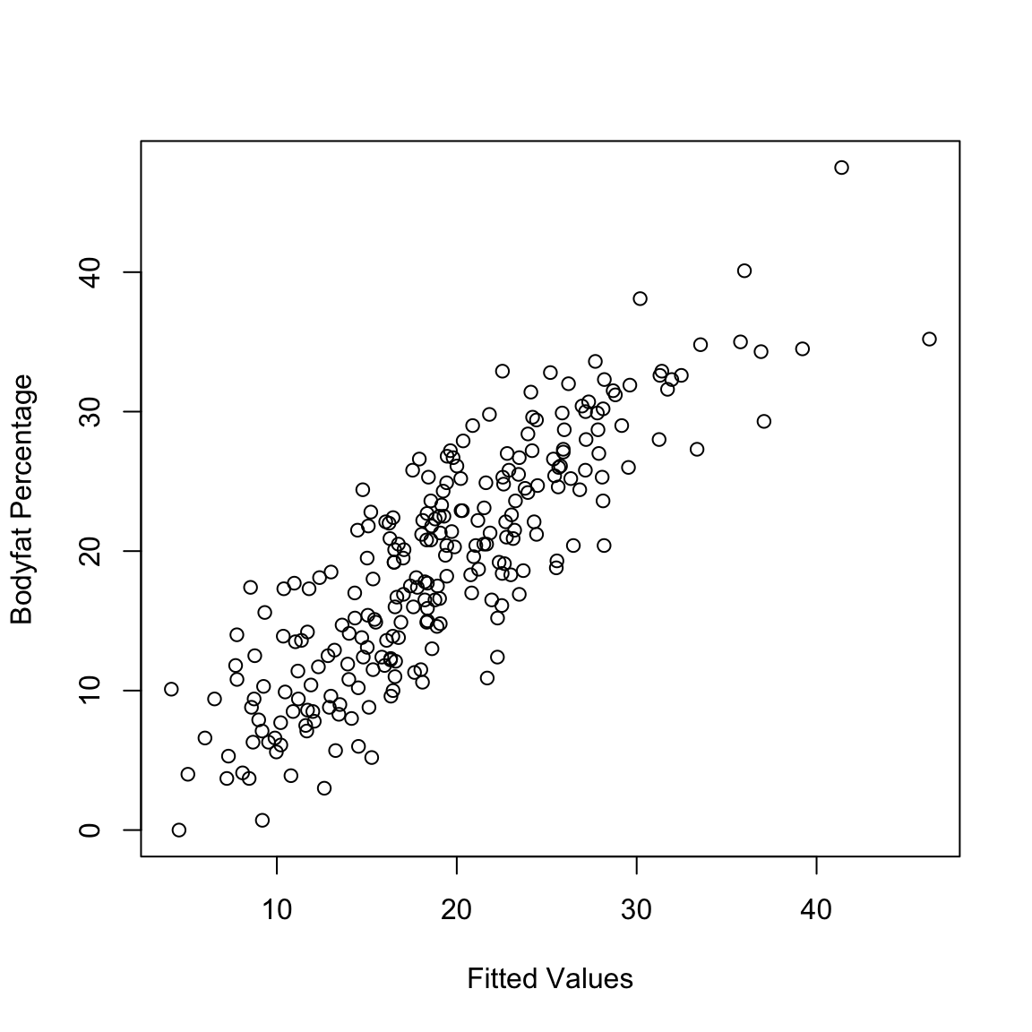
We can quantify how good of a fit our model is by taking the correlation between these two values. Specifically, the square of the correlation of \(y\) and \(\hat{y}\) is known as the Coefficient of
Determination or Multiple \(R^2\) or simply \(R^2\):
\[\begin{equation*}
R^2 = \left(cor(y_i,\hat{y}_i ) \right)^2.
\end{equation*}\]
This is an important
and widely used measure of the effectiveness of the regression
equation and given in our summary the lm fit.
## [1] 0.7265596##
## Call:
## lm(formula = BODYFAT ~ ., data = body)
##
## Residuals:
## Min 1Q Median 3Q Max
## -11.0729 -3.2387 -0.0782 3.0623 10.3611
##
## Coefficients:
## Estimate Std. Error t value Pr(>|t|)
## (Intercept) -3.748e+01 1.449e+01 -2.585 0.01031 *
## AGE 1.202e-02 2.934e-02 0.410 0.68246
## WEIGHT -1.392e-01 4.509e-02 -3.087 0.00225 **
## HEIGHT -1.028e-01 9.787e-02 -1.051 0.29438
## CHEST -8.312e-04 9.989e-02 -0.008 0.99337
## ABDOMEN 9.685e-01 8.531e-02 11.352 < 2e-16 ***
## HIP -1.834e-01 1.448e-01 -1.267 0.20648
## THIGH 2.857e-01 1.362e-01 2.098 0.03693 *
## ---
## Signif. codes: 0 '***' 0.001 '**' 0.01 '*' 0.05 '.' 0.1 ' ' 1
##
## Residual standard error: 4.438 on 244 degrees of freedom
## Multiple R-squared: 0.7266, Adjusted R-squared: 0.7187
## F-statistic: 92.62 on 7 and 244 DF, p-value: < 2.2e-16A high value of \(R^2\) means that the fitted values (given by the fitted regression equation) are close to the observed values and hence indicates that the regression equation fits the data well. A low value, on the other hand, means that the fitted values are far from the observed values and hence the regression line does not fit the data well.
Note that \(R^2\) has no units (because its a correlation). In other words, it is scale-free.
6.4.2 Residuals and Residual Sum of Squares (RSS)
For every point in the scatter the error we make in our prediction on a specific observation is the residual and is
defined as
\[\begin{equation*}
r_i = y_i-\hat{y}_i
\end{equation*}\]
Residuals are again so important that \(lm()\) automatically calculates them for us and they are contained in the lm object created.
## 1 2 3 4 5 6
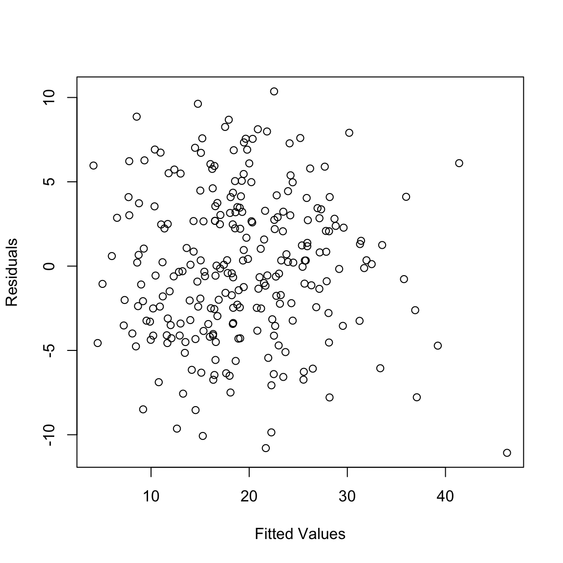
## -4.026695 -4.120189 6.874004 -1.495017 2.724355 4.614712A common way of looking at the residuals is to plot them against the fitted values.
 One can also plot the residuals against each of the explanatory
variables (note we didn’t remove the outliers in our regression so we include them in our plots).
One can also plot the residuals against each of the explanatory
variables (note we didn’t remove the outliers in our regression so we include them in our plots).
par(mfrow = c(3, 3))
for (i in 2:8) {
    plot(body[, i], ft$residuals, xlab = names(body)[i],
        ylab = "Residuals")
}
par(mfrow = c(1, 1))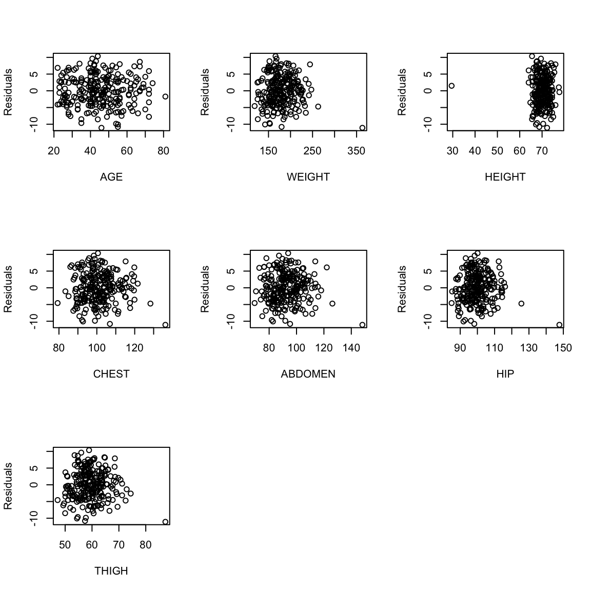
The residuals represent what is left in the response (\(y\)) after all the linear effects of the explanatory variables are taken out.
One consequence of this is that the residuals are uncorrelated with every explanatory variable. We can check this in easily in the body fat example.
for (i in 2:8) {
    cat("Correlation with", names(body)[i], ":\t")
    cat(cor(body[, i], residuals(ft)), "\n")
}
## Correlation with AGE : -1.754044e-17
## Correlation with WEIGHT : 4.71057e-17
## Correlation with HEIGHT : -1.720483e-15
## Correlation with CHEST : -4.672628e-16
## Correlation with ABDOMEN : -7.012368e-16
## Correlation with HIP : -8.493675e-16
## Correlation with THIGH : -5.509094e-16Moreover, as we discussed in simple regression, the residuals always have mean zero:
## [1] 2.467747e-16Again, these are automatic properties of any least-squares regression. This is not evidence that you have a good fit or that model makes sense!
Also, if one were to fit a regression equation to the residuals in terms of the same explanatory variables, then the fitted regression equation will have all coefficients exactly equal to zero:
m.res = lm(ft$residuals ~ body$AGE + body$WEIGHT +
    body$HEIGHT + body$CHEST + body$ABDOMEN + body$HIP +
    body$THIGH)
summary(m.res)
##
## Call:
## lm(formula = ft$residuals ~ body$AGE + body$WEIGHT + body$HEIGHT +
## body$CHEST + body$ABDOMEN + body$HIP + body$THIGH)
##
## Residuals:
## Min 1Q Median 3Q Max
## -11.0729 -3.2387 -0.0782 3.0623 10.3611
##
## Coefficients:
## Estimate Std. Error t value Pr(>|t|)
## (Intercept) 2.154e-14 1.449e+01 0 1
## body$AGE 1.282e-17 2.934e-02 0 1
## body$WEIGHT 1.057e-16 4.509e-02 0 1
## body$HEIGHT -1.509e-16 9.787e-02 0 1
## body$CHEST 1.180e-16 9.989e-02 0 1
## body$ABDOMEN -2.452e-16 8.531e-02 0 1
## body$HIP -1.284e-16 1.448e-01 0 1
## body$THIGH -1.090e-16 1.362e-01 0 1
##
## Residual standard error: 4.438 on 244 degrees of freedom
## Multiple R-squared: 6.384e-32, Adjusted R-squared: -0.02869
## F-statistic: 2.225e-30 on 7 and 244 DF, p-value: 1If the regression equation fits the data well, the residuals are supposed to be small. One popular way of assessing the size of the residuals is to compute their sum of squares. This quantity is called the Residual Sum of Squares (RSS).
## [1] 4806.806Note that RSS depends on the units in which the response variable is measured.
Relationship to \(R^2\)
There is a very simple relationship between RSS and \(R^2\) (recall that \(R^2\) is the square of the correlation between the response values and the fitted values): \[\begin{equation*} R^2 = 1 - \frac{RSS}{TSS} \end{equation*}\] where TSS stands for Total Sum of Squares and is defined as \[\begin{equation*} TSS = \sum_{i=1}^n \left(y_i - \bar{y} \right)^2. \end{equation*}\] TSS is just the variance of y without the \(1/(n-1)\) term.
It is easy to verify this formula in R.
## [1] 4806.806## [1] 0.7265596##
## Call:
## lm(formula = BODYFAT ~ ., data = body)
##
## Residuals:
## Min 1Q Median 3Q Max
## -11.0729 -3.2387 -0.0782 3.0623 10.3611
##
## Coefficients:
## Estimate Std. Error t value Pr(>|t|)
## (Intercept) -3.748e+01 1.449e+01 -2.585 0.01031 *
## AGE 1.202e-02 2.934e-02 0.410 0.68246
## WEIGHT -1.392e-01 4.509e-02 -3.087 0.00225 **
## HEIGHT -1.028e-01 9.787e-02 -1.051 0.29438
## CHEST -8.312e-04 9.989e-02 -0.008 0.99337
## ABDOMEN 9.685e-01 8.531e-02 11.352 < 2e-16 ***
## HIP -1.834e-01 1.448e-01 -1.267 0.20648
## THIGH 2.857e-01 1.362e-01 2.098 0.03693 *
## ---
## Signif. codes: 0 '***' 0.001 '**' 0.01 '*' 0.05 '.' 0.1 ' ' 1
##
## Residual standard error: 4.438 on 244 degrees of freedom
## Multiple R-squared: 0.7266, Adjusted R-squared: 0.7187
## F-statistic: 92.62 on 7 and 244 DF, p-value: < 2.2e-16If we did not have any explanatory variables, then we would predict the value of bodyfat percentage for any individual by simply the mean of the bodyfat values in our sample. The total squared error for this prediction is given by TSS. On the other hand, the total squared error for the prediction using linear regression based on the explanatory variables is given by RSS. Therefore \(1 - R^2\) represents the reduction in the squared error because of the explanatory variables.
6.4.3 Behaviour of RSS (and \(R^2\)) when variables are added or removed from the regression equation
The value of RSS always increases when one or more explanatory variables are removed from the regression equation. For example, suppose that we remove the variable abdomen circumference from the regression equation. The new RSS will then be:
ft.1 = lm(BODYFAT ~ AGE + WEIGHT + HEIGHT + CHEST +
    HIP + THIGH, data = body)
rss.ft1 = summary(ft.1)$r.squared
rss.ft1
## [1] 0.5821305## Length Class Mode
## 0 NULL NULLNotice that there is a quite a lot of increase in the RSS. What if we had kept ABDOMEN in the model but dropped the variable CHEST?
ft.2 = lm(BODYFAT ~ AGE + WEIGHT + HEIGHT + ABDOMEN +
    HIP + THIGH, data = body)
rss.ft2 = summary(ft.2)$r.squared
rss.ft2
## [1] 0.7265595## [1] 4806.806The RSS again increases but by a very very small amount. This therefore suggests that Abdomen circumference is a more important variable in this regression compared to Chest circumference.
The moral of this exercise is the following. The RSS always increases when variables are dropped from the regression equation. However the amount of increase varies for different variables. We can understand the importance of variables in a multiple regression equation by noting the amount by which the RSS increases when the individual variables are dropped. We will come back to this point while studying inference in the multiple regression model.
Because RSS has a direct relation to \(R^2\) via \(R^2 = 1 - (RSS/TSS)\), one can see \(R^2\) decreases when variables are removed from the model. However the amount of decrease will be different for different variables. For example, in the body fat dataset, after removing the abdomen circumference variable, \(R^2\) changes to:
ft.1 = lm(BODYFAT ~ AGE + WEIGHT + HEIGHT + CHEST +
    HIP + THIGH, data = body)
R2.ft1 = summary(ft.1)$r.squared
R2.ft1
## [1] 0.5821305## [1] 0.7265596Notice that there is a lot of decrease in \(R^2\). What happens if the variable Chest circumference is dropped.
ft.2 = lm(BODYFAT ~ AGE + WEIGHT + HEIGHT + ABDOMEN +
    HIP + THIGH, data = body)
R2.ft2 = summary(ft.2)$r.squared
R2.ft2
## [1] 0.7265595## [1] 0.7265596There is now a very very small decrease.
6.4.4 Residual Degrees of Freedom and Residual Standard Error
In a regression with \(p\) explanatory variables, the residual degrees of freedom is given by \(n - p - 1\) (recall that \(n\) is the number of observations). This can be thought of as the effective number of residuals. Even though there are \(n\) residuals, they are supposed to satisfy \(p+1\) exact equations (they sum to zero and they have zero correlation with each of the \(p\) explanatory variables).
The Residual Standard Error is defined as: \[\begin{equation*} \sqrt{\frac{\text{Residual Sum of Squares}}{\text{Residual Degrees of Freedom}}} \end{equation*}\] This can be interpreted as the average magnitude of an individual residual and can be used to assess the sizes of residuals (in particular, to find and identify large residual values).
For illustration,
ft = lm(BODYFAT ~ AGE + WEIGHT + HEIGHT + CHEST + ABDOMEN +
    HIP + THIGH, data = body)
n = nrow(body)
p = 7
rs.df = n - p - 1
rs.df
## [1] 244ft = lm(BODYFAT ~ AGE + WEIGHT + HEIGHT + CHEST + ABDOMEN +
HIP + THIGH, data = body)
rss = sum((ft$residuals)^2)
rse = sqrt(rss/rs.df)
rse## [1] 4.438471Both of these are printed in the summary function in R:
##
## Call:
## lm(formula = BODYFAT ~ AGE + WEIGHT + HEIGHT + CHEST + ABDOMEN +
##     HIP + THIGH, data = body)
##
## Residuals:
##      Min       1Q   Median       3Q      Max
## -11.0729  -3.2387  -0.0782   3.0623  10.3611
##
## Coefficients:
##               Estimate Std. Error t value Pr(>|t|)
## (Intercept) -3.748e+01  1.449e+01  -2.585  0.01031 *
## AGE          1.202e-02  2.934e-02   0.410  0.68246
## WEIGHT      -1.392e-01  4.509e-02  -3.087  0.00225 **
## HEIGHT      -1.028e-01  9.787e-02  -1.051  0.29438
## CHEST       -8.312e-04  9.989e-02  -0.008  0.99337
## ABDOMEN      9.685e-01  8.531e-02  11.352  < 2e-16 ***
## HIP         -1.834e-01  1.448e-01  -1.267  0.20648
## THIGH        2.857e-01  1.362e-01   2.098  0.03693 *
## ---
## Signif. codes:  0 '***' 0.001 '**' 0.01 '*' 0.05 '.' 0.1 ' ' 1
##
## Residual standard error: 4.438 on 244 degrees of freedom
## Multiple R-squared:  0.7266, Adjusted R-squared:  0.7187
## F-statistic: 92.62 on 7 and 244 DF,  p-value: < 2.2e-16
6.5 Multiple Regression With Categorical Explanatory Variables
In many instances of regression, some of the explanatory variables are categorical (note that the response variable is always continuous). For example, consider the (short version of the) college dataset that you have already encountered.
We can do a regression here with the retention rate (variable name
RET-FT4) as the response and all other variables as the
explanatory variables. Note that one of the explanatory variables
(variable name CONTROL) is categorical. This variable represents whether
the college is public (1), private non-profit (2) or private for
profit (3). Dealing with such categorical variables is a little
tricky. To illustrate the ideas here, let us focus on a regression for
the retention rate based on just two explanatory variables: the
out-of-state tuition and the categorical variable CONTROL.
The important thing to note about the variable CONTROL is that
its levels 1, 2 and 3 are completely arbitrary and have no
particular meaning. For example, we could have called its levels \(A\),
\(B\), \(C\) or \(Pu\), \(Pr-np\), \(Pr-fp\) as well. If we use the \(lm()\)
function in the usual way with TUITIONFEE and CONTROL
as the explanatory variables, then R will treat CONTROL as a
continuous variable which does not make sense:
##
## Call:
## lm(formula = RET_FT4 ~ TUITIONFEE_OUT + CONTROL, data = scorecard)
##
## Residuals:
##      Min       1Q   Median       3Q      Max
## -0.69041 -0.04915  0.00516  0.05554  0.33165
##
## Coefficients:
##                  Estimate Std. Error t value Pr(>|t|)
## (Intercept)     6.661e-01  9.265e-03   71.90   <2e-16 ***
## TUITIONFEE_OUT  9.405e-06  3.022e-07   31.12   <2e-16 ***
## CONTROL        -8.898e-02  5.741e-03  -15.50   <2e-16 ***
## ---
## Signif. codes:  0 '***' 0.001 '**' 0.01 '*' 0.05 '.' 0.1 ' ' 1
##
## Residual standard error: 0.08741 on 1238 degrees of freedom
## Multiple R-squared:  0.4391, Adjusted R-squared:  0.4382
## F-statistic: 484.5 on 2 and 1238 DF,  p-value: < 2.2e-16
The regression coefficient for CONTROL has the usual
interpretation (if CONTROL increases by one unit, \(\dots\)) which
does not make much sense because CONTROL is categorical and so
increasing it by one unit is nonsensical. So everything about this regression is wrong (and we shouldn’t interpret anything from the inference here).
You can check that R is
treating CONTROL as a numeric variable by:
## [1] TRUEThe correct way to deal with categorical variables in R is to treat them as factors:
##
## Call:
## lm(formula = RET_FT4 ~ TUITIONFEE_OUT + as.factor(CONTROL), data = scorecard)
##
## Residuals:
##      Min       1Q   Median       3Q      Max
## -0.68856 -0.04910  0.00505  0.05568  0.33150
##
## Coefficients:
##                       Estimate Std. Error t value Pr(>|t|)
## (Intercept)          5.765e-01  7.257e-03  79.434  < 2e-16 ***
## TUITIONFEE_OUT       9.494e-06  3.054e-07  31.090  < 2e-16 ***
## as.factor(CONTROL)2 -9.204e-02  5.948e-03 -15.474  < 2e-16 ***
## as.factor(CONTROL)3 -1.218e-01  3.116e-02  -3.909 9.75e-05 ***
## ---
## Signif. codes:  0 '***' 0.001 '**' 0.01 '*' 0.05 '.' 0.1 ' ' 1
##
## Residual standard error: 0.08732 on 1237 degrees of freedom
## Multiple R-squared:  0.4408, Adjusted R-squared:  0.4394
## F-statistic:   325 on 3 and 1237 DF,  p-value: < 2.2e-16
We can make this output a little better by fixing up the factor, rather than having R make it a factor on the fly:
scorecard$CONTROL <- factor(scorecard$CONTROL, levels = c(1,
    2, 3), labels = c("public", "private", "private for-profit"))
req = lm(RET_FT4 ~ TUITIONFEE_OUT + CONTROL, data = scorecard)
summary(req)
##
## Call:
## lm(formula = RET_FT4 ~ TUITIONFEE_OUT + CONTROL, data = scorecard)
##
## Residuals:
## Min 1Q Median 3Q Max
## -0.68856 -0.04910 0.00505 0.05568 0.33150
##
## Coefficients:
## Estimate Std. Error t value Pr(>|t|)
## (Intercept) 5.765e-01 7.257e-03 79.434 < 2e-16 ***
## TUITIONFEE_OUT 9.494e-06 3.054e-07 31.090 < 2e-16 ***
## CONTROLprivate -9.204e-02 5.948e-03 -15.474 < 2e-16 ***
## CONTROLprivate for-profit -1.218e-01 3.116e-02 -3.909 9.75e-05 ***
## ---
## Signif. codes: 0 '***' 0.001 '**' 0.01 '*' 0.05 '.' 0.1 ' ' 1
##
## Residual standard error: 0.08732 on 1237 degrees of freedom
## Multiple R-squared: 0.4408, Adjusted R-squared: 0.4394
## F-statistic: 325 on 3 and 1237 DF, p-value: < 2.2e-16What do you notice that is different than our wrong output when the CONTROL variable was treated as numeric?
Why is the coefficient of TUITIONFEE so small?
6.5.1 Separate Intercepts: The coefficients of Categorical/Factor variables
What do the multiple coefficients mean for the variable CONTROL?
This equation can be written in full as:
\[\begin{equation*}
RET = 0.5765 + 9.4\times 10^{-6}*TUITIONFEE
-0.0092*I\left(CONTROL = 2 \right) -
0.1218*I\left(CONTROL = 3 \right).
\end{equation*}\]
The variable \(I\left(CONTROL = 2 \right)\) is the indicator function, which takes the value 1 if the
college has CONTROL equal to 2 (i.e., if the college is private
non-profit) and 0 otherwise. Similarly the variable \(I\left(CONTROL = 3 \right)\) takes the value 1 if the college has CONTROL equal to 3
(i.e., if the college is private for profit) and 0
otherwise. Variables which take only the two values 0 and 1 are called
indicator variables.
Note that the variable \(I\left(CONTROL = 1 \right)\) does not appear in the regression equation . This means that the level 1 (i.e., the college is public) is the baseline level here and the effects of \(-0.0092\) and \(0.1218\) for private for-profit and private non-profit colleges respectively should be interpreted relative to public colleges.
The regression equation can effectively be broken down into three equations. For public colleges, the two indicator variables in are zero and the equation becomes: \[\begin{equation*} RET = 0.5765 + 9.4\times 10^{-6}*TUITIONFEE. \end{equation*}\] For private non-profit colleges, the equation becomes \[\begin{equation*} RET = 0.5673 + 9.4\times 10^{-6}*TUITIONFEE. \end{equation*}\] and for private for-profit colleges, \[\begin{equation*} RET = 0.4547 + 9.4\times 10^{-6}*TUITIONFEE. \end{equation*}\]
Note that the coefficient of TUITIONFEE is the same in each of these
equations (only the intercept changes). We can plot a scatterplot
together with all these lines.
cols <- c("blue", "red", "black")
plot(RET_FT4 ~ TUITIONFEE_OUT, data = scorecard, xlab = "Tuition Fee (out of state)",
    ylab = "Retention Rate", col = cols[scorecard$CONTROL])
baseline <- coef(req)[["(Intercept)"]]
slope <- coef(req)[["TUITIONFEE_OUT"]]
for (ii in 1:nlevels(scorecard$CONTROL)) {
    lev <- levels(scorecard$CONTROL)[[ii]]
    if (ii == 1) {
        abline(a = baseline, b = slope, col = cols[[ii]])
    }
    else {
        abline(a = baseline + coef(req)[[ii + 1]],
            b = slope, col = cols[[ii]])
    }
}
legend("bottomright", levels(scorecard$CONTROL), fill = cols)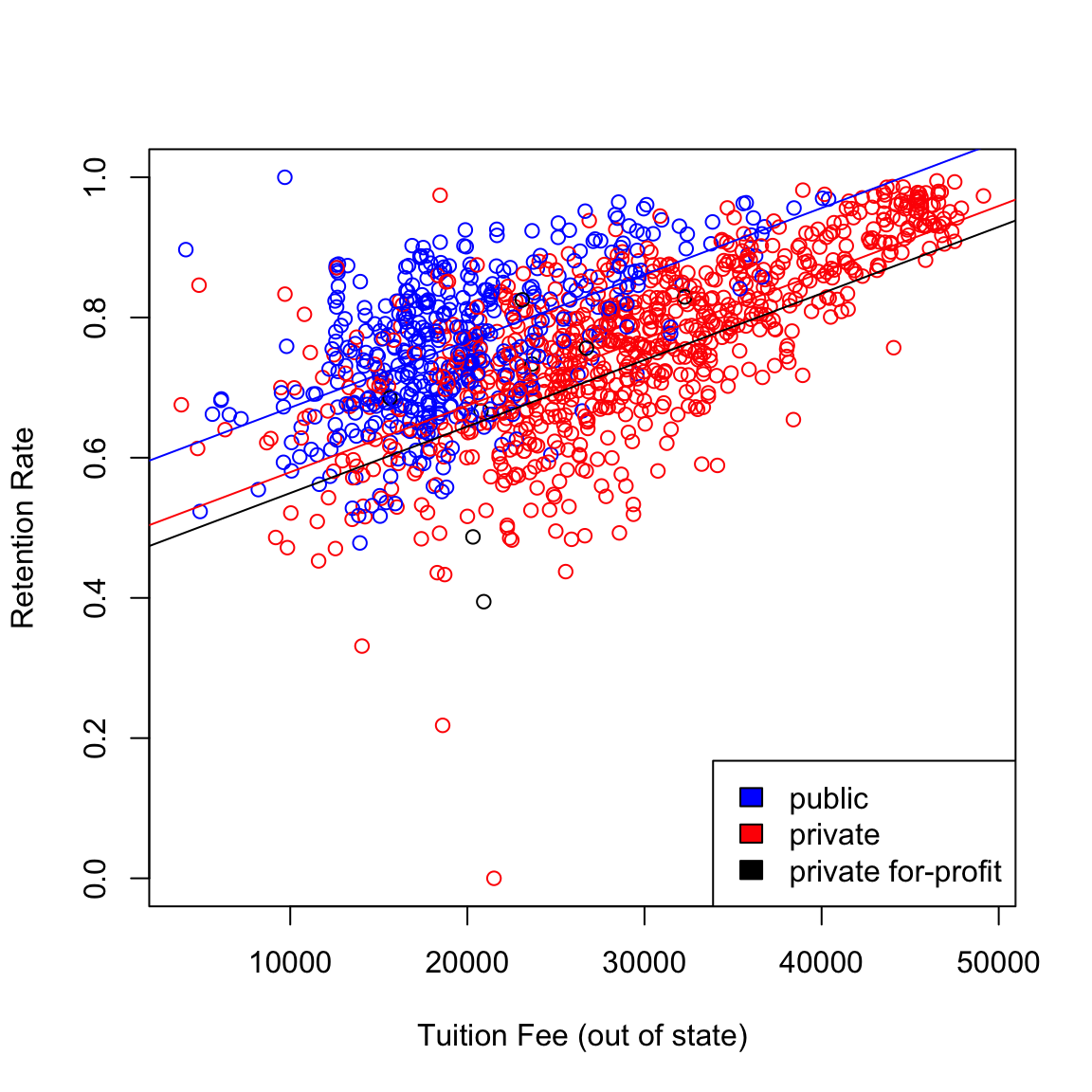
6.5.2 Separate Slopes: Interactions
What if we want these regression equations to have different slopes as well as different intercepts for each of the types of colleges?
Intuitively, we can do separate regressions for each of the three groups given by
the CONTROL variable.
Alternatively, we can do this in multiple
regression by adding an interaction variable between CONTROL and
TUITIONFEE as follows:
req.1 = lm(RET_FT4 ~ TUITIONFEE_OUT + CONTROL + TUITIONFEE_OUT:CONTROL,
    data = scorecard)
summary(req.1)
##
## Call:
## lm(formula = RET_FT4 ~ TUITIONFEE_OUT + CONTROL + TUITIONFEE_OUT:CONTROL,
## data = scorecard)
##
## Residuals:
## Min 1Q Median 3Q Max
## -0.68822 -0.04982 0.00491 0.05555 0.32900
##
## Coefficients:
## Estimate Std. Error t value Pr(>|t|)
## (Intercept) 5.814e-01 1.405e-02 41.372 < 2e-16
## TUITIONFEE_OUT 9.240e-06 6.874e-07 13.441 < 2e-16
## CONTROLprivate -9.830e-02 1.750e-02 -5.617 2.4e-08
## CONTROLprivate for-profit -2.863e-01 1.568e-01 -1.826 0.0681
## TUITIONFEE_OUT:CONTROLprivate 2.988e-07 7.676e-07 0.389 0.6971
## TUITIONFEE_OUT:CONTROLprivate for-profit 7.215e-06 6.716e-06 1.074 0.2829
##
## (Intercept) ***
## TUITIONFEE_OUT ***
## CONTROLprivate ***
## CONTROLprivate for-profit .
## TUITIONFEE_OUT:CONTROLprivate
## TUITIONFEE_OUT:CONTROLprivate for-profit
## ---
## Signif. codes: 0 '***' 0.001 '**' 0.01 '*' 0.05 '.' 0.1 ' ' 1
##
## Residual standard error: 0.08734 on 1235 degrees of freedom
## Multiple R-squared: 0.4413, Adjusted R-squared: 0.4391
## F-statistic: 195.1 on 5 and 1235 DF, p-value: < 2.2e-16Note that this regression equation has two more coefficients compared to the previous regression (which did not have the interaction term). The two additional variables are the product of the terms of each of the previous terms: \(TUITIONFEE * I(CONTROL = 2)\) and \(TUITIONFEE * I(CONTROL = 3)\).
The presence of these product terms means that three separate slopes per each level of the factor are being fit here, why?
Alternatively, this regression with interaction can also be done in R via:
##
## Call:
## lm(formula = RET_FT4 ~ TUITIONFEE_OUT * CONTROL, data = scorecard)
##
## Residuals:
##      Min       1Q   Median       3Q      Max
## -0.68822 -0.04982  0.00491  0.05555  0.32900
##
## Coefficients:
##                                            Estimate Std. Error t value Pr(>|t|)
## (Intercept)                               5.814e-01  1.405e-02  41.372  < 2e-16
## TUITIONFEE_OUT                            9.240e-06  6.874e-07  13.441  < 2e-16
## CONTROLprivate                           -9.830e-02  1.750e-02  -5.617  2.4e-08
## CONTROLprivate for-profit                -2.863e-01  1.568e-01  -1.826   0.0681
## TUITIONFEE_OUT:CONTROLprivate             2.988e-07  7.676e-07   0.389   0.6971
## TUITIONFEE_OUT:CONTROLprivate for-profit  7.215e-06  6.716e-06   1.074   0.2829
##
## (Intercept)                              ***
## TUITIONFEE_OUT                           ***
## CONTROLprivate                           ***
## CONTROLprivate for-profit                .
## TUITIONFEE_OUT:CONTROLprivate
## TUITIONFEE_OUT:CONTROLprivate for-profit
## ---
## Signif. codes:  0 '***' 0.001 '**' 0.01 '*' 0.05 '.' 0.1 ' ' 1
##
## Residual standard error: 0.08734 on 1235 degrees of freedom
## Multiple R-squared:  0.4413, Adjusted R-squared:  0.4391
## F-statistic: 195.1 on 5 and 1235 DF,  p-value: < 2.2e-16
The three separate regressions can be plotted in one plot as before.
cols <- c("blue", "red", "black")
plot(RET_FT4 ~ TUITIONFEE_OUT, data = scorecard, xlab = "Tuition Fee (out of state)",
    ylab = "Retention Rate", col = cols[scorecard$CONTROL])
baseline <- coef(req.1)[["(Intercept)"]]
slope <- coef(req.1)[["TUITIONFEE_OUT"]]
for (ii in 1:nlevels(scorecard$CONTROL)) {
    lev <- levels(scorecard$CONTROL)[[ii]]
    if (ii == 1) {
        abline(a = baseline, b = slope, col = cols[[ii]])
    }
    else {
        abline(a = baseline + coef(req.1)[[ii + 1]],
            b = slope + coef(req.1)[[ii + 3]], col = cols[[ii]])
    }
}
legend("bottomright", levels(scorecard$CONTROL), fill = cols)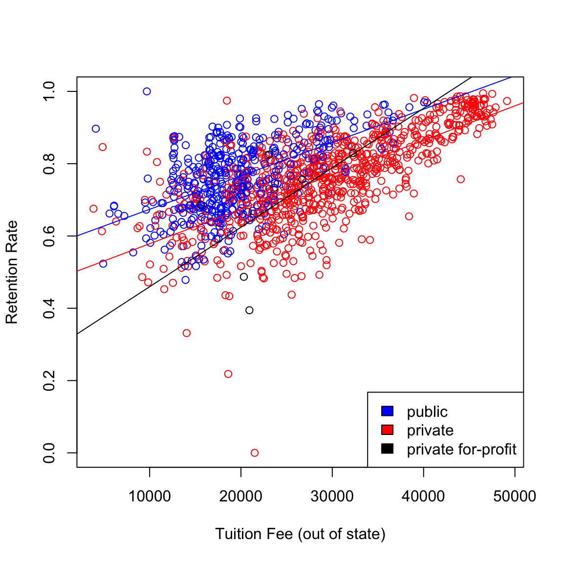
Interaction terms make regression equations complicated (have more variables) and also slightly harder to interpret although, in some situations, they really improve predictive power. In this particular example, note that the multiple \(R^2\) only increased from 0.4408 to 0.4413 after adding the interaction terms. This small increase means that the interaction terms are not really adding much to the regression equation so we are better off using the previous model with no interaction terms.
To get more practice with regressions having categorical variables, let us consider the bike sharing dataset discussed above.
Let us fit a basic regression equation with casual (number of
bikes rented by casual users hourly) as the response variable and the
explanatory variables being atemp (normalized feeling
temperature), workingday. For this dataset, I’ve already encoded the categorical variables as factors.
##    Min. 1st Qu.  Median    Mean 3rd Qu.    Max.
## 0.07907 0.33784 0.48673 0.47435 0.60860 0.84090## No Yes
## 231 500## Clear/Partly Cloudy Light Rain/Snow Misty
## 463 21 247We fit the regression equation with a different shift in the mean for each level:
##
## Call:
## lm(formula = casual ~ atemp + workingday + weathersit, data = bike)
##
## Residuals:
##      Min       1Q   Median       3Q      Max
## -1456.76  -243.97   -22.93   166.81  1907.20
##
## Coefficients:
##                           Estimate Std. Error t value Pr(>|t|)
## (Intercept)                 350.31      55.11   6.357 3.63e-10 ***
## atemp                      2333.77      97.48  23.942  < 2e-16 ***
## workingdayYes              -794.11      33.95 -23.388  < 2e-16 ***
## weathersitLight Rain/Snow  -523.79      95.23  -5.500 5.26e-08 ***
## weathersitMisty            -150.79      33.75  -4.468 9.14e-06 ***
## ---
## Signif. codes:  0 '***' 0.001 '**' 0.01 '*' 0.05 '.' 0.1 ' ' 1
##
## Residual standard error: 425.2 on 726 degrees of freedom
## Multiple R-squared:  0.6186, Adjusted R-squared:  0.6165
## F-statistic: 294.3 on 4 and 726 DF,  p-value: < 2.2e-16
How are the coefficients in the above regression interpreted?
There are interactons that one
can add here too. For example, I can add an interaction between
workingday and atemp:
##
## Call:
## lm(formula = casual ~ atemp + workingday + weathersit + workingday:atemp,
##     data = bike)
##
## Residuals:
##      Min       1Q   Median       3Q      Max
## -1709.76  -198.09   -55.12   152.88  1953.07
##
## Coefficients:
##                           Estimate Std. Error t value Pr(>|t|)
## (Intercept)                -276.22      77.48  -3.565 0.000388 ***
## atemp                      3696.41     155.56  23.762  < 2e-16 ***
## workingdayYes               166.71      94.60   1.762 0.078450 .
## weathersitLight Rain/Snow  -520.78      88.48  -5.886 6.05e-09 ***
## weathersitMisty            -160.28      31.36  -5.110 4.12e-07 ***
## atemp:workingdayYes       -2052.09     190.48 -10.773  < 2e-16 ***
## ---
## Signif. codes:  0 '***' 0.001 '**' 0.01 '*' 0.05 '.' 0.1 ' ' 1
##
## Residual standard error: 395.1 on 725 degrees of freedom
## Multiple R-squared:  0.6712, Adjusted R-squared:  0.6689
## F-statistic:   296 on 5 and 725 DF,  p-value: < 2.2e-16
What is the interpretation of the coefficients now?
6.6 Inference in Multiple Regression
So far, we have learned how to fit multiple regression equations to observed data and interpret the coefficient. Inference is necessary for answering questions such as: “Is the observed relationship between the response and the explanatory variables real or is it merely caused by sampling variability?”
We will again consider both parametric models and resampling techniques for inference.
6.6.1 Parametric Models for Inference
There is a response variable \(y\) and \(p\) explanatory variables \(x^{(1)}, \dots, x^{(p)}\). The data generation model is similar to that of simple regression: \[\begin{equation*} y = \beta_0 + \beta_1 x^{(1)} + \dots + \beta_p x^{(p)} + e. \end{equation*}\] The numbers \(\beta_0, \dots, \beta_p\) are the parameters of the model and unknown.
The error \(e\) is the only random part of the model, and we make the same assumptions as in simple regression:
- \(e_i\) are independent for each observation \(i\)
- \(e_i\) all have the same distribution with mean \(0\) and variance \(\sigma^2\)
- \(e_i\) follow a normal distribution
We could write this more succinctly as \[e_i \text{ are i.i.d } N(0,\sigma^2)\] but it’s helpful to remember that these are separate assumptions, so we can talk about which are the most important.
This means that under this model, \[y \sim N(\beta_0 + \beta_1 x^{(1)} + \dots + \beta_p x^{(p)}, \sigma^2)\] i.e. the observed \(y_i\) are normal and independent from each other, but each with a different mean, which depends on \(x_i\) (so the \(y_i\) are NOT i.i.d. because not identically distributed).
Estimates
The numbers \(\beta_0, \dots, \beta_p\) capture the true relationship between \(y\) and \(x_1, \dots, x_p\). Also unknown is the quantity \(\sigma^2\) which is the variance of the unknown \(e_i\). When we fit a regression equation to a dataset via \(lm()\) in R, we obtain estimates \(\hat{\beta}_j\) of the unknown \(\beta_j\).
The residual \(r_i\) serve as natural proxies for the unknown random errors \(e_i\). Therefore a natural estimate for the error standard deviation \(\sigma\) is the Residual Standard Error, \[\hat{\sigma}^2=\frac{1}{n-p-1}\sum r_i^2=\frac{1}{n-p-1} RSS\] Notice this is the same as our previous equation from simple regression, only now we are using \(n-p-1\) as our correction to make the estimate unbiased.
6.6.2 Global Fit
The most obvious question is the global question: are these variables cummulatively any good in predicting \(y\)? This can be restated as, whether you could predict \(y\) just as well if didn’t use any of the \(x^{(j)}\) variables.
If we didn’t use any of the variables, what is our best “prediction” of \(y\)?
So our question can be phrased as whether our prediction that we estimated, \(\hat{y}(x)\), is better than just \(\bar{y}\) in predicting \(y\).
Equivalently, we can think that our null hypothesis is \[H_0: \beta_j=0, \text{for all }j\]
6.6.2.1 Parametric Test of Global Fit
The parametric test that is commonly used for assessing the global fit is a F-test. A common way to assess the fit, we have just said is either large \(R^2\) or small \(RSS=\sum_{i=1}^{n}r_i^2\).
We can also think our global test is an implicit test for comparing two possible prediction models
Model 0: No variables, just predict \(\bar{y}\) for all observations
Model 1: Our linear model with all the variables
Then we could also say that we could test the global fit by comparing the RSS from model 0 (the null model), versus model 1 (the one with the variables), e.g. \[RSS_0-RSS_1\]
This will always be positive, why?
We will actually instead change this to be a proportional increase, i.e. relative to the full model, how much increase in RSS do I get when I take out the variables: \[\frac{RSS_0-RSS_1}{RSS_1}\]
To make this quantity more comparable across many datasets, we are going to normalize this quantity by the number of variables in the data, \[F=\frac{(RSS_0-RSS_1)/p}{RSS_1/(n-p-1)}\] Notice that the \(RSS_0\) of our 0 model is actually the TSS. This is because \[\hat{y}^{\text{Model 0}}=\bar{y}\] so \[RSS_0=\sum_{i=1}^n (y_i-\hat{y}^{\text{Model 0}})^2=\sum_{i=1}^n (y_i-\bar{y})^2\] Further, \[RSS_1/(n-p-1)=\hat{\sigma}^2\] So we have \[F=\frac{(TSS-RSS)/p}{\hat{\sigma}^2}\]
All of this we can verify on our data:
n <- nrow(body)
p <- ncol(body) - 1
tss <- (n - 1) * var(body$BODYFAT)
rss <- sum(residuals(ft)^2)
sigma <- summary(ft)$sigma
(tss - rss)/p/sigma^2
## [1] 92.61904## value numdf dendf
## 92.61904 7.00000 244.00000We do all this normalization, because under our assumptions of the parametric model, the \(F\) statistic above follows a \(F\)-distribution. The \(F\) distribution you have seen in a HW when you were simulating data, and has two parameters, the degrees of freedom of the numerator (\(df1\)) and the degrees of freedom of the denominator (\(df2\)); they are those constants we divide the numerator and denominator by in the definition of the \(F\) statistic. Then the \(F\) statistic we described above follows a \(F(p, n-p-1)\) distribution under our parametric model.
Here is the null distribution for our \(F\) statistic for the bodyfat:
curve(df(x, df1 = p, df2 = n - p - 1), xlim = c(0,
    5), main = paste("F(", p, ",", n - p - 1, ") distribution"),
    sub = paste("Observed:", round(summary(ft)$fstatistic["value"],
        2)))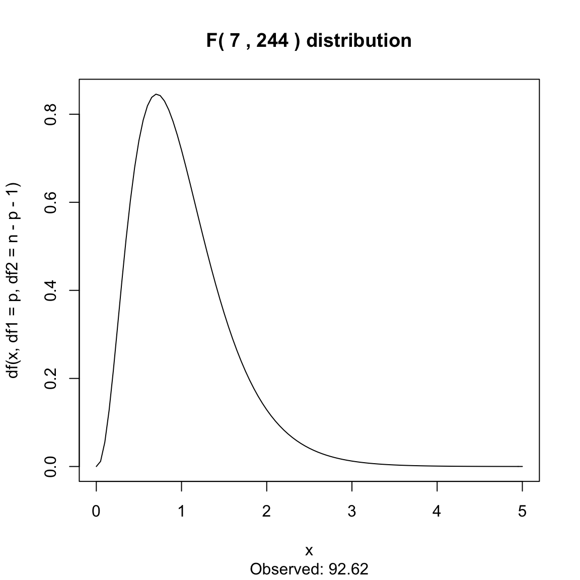
This is a highly significant result, and indeed most tests of general fit are highly significant. It is rare that the entire set of variables collected have zero predictive value to the response!
6.6.2.2 Permutation test for global fit
Our null hypothesis to assess the global fit is that the \(x_i\) do not give us any information regarding the \(y\). We had a similar situation previously when we considered comparing two groups. There, we measured a response \(y\) on two groups, and wanted to know whether the group assignment of the observation made a difference in the \(y\) response. To answer that question with permutation tests, we permuted the assignment of the \(y_i\) variables into the two groups.
Then we can think of the global fit of the regression similarly, since under the null knowing \(x_i\) doesn’t give us any information about \(y_i\), so I can permute the assignment of the \(y_i\) to \(x_i\) and it shouldn’t change the fit of our data.
Specifically, we have a statistic, \(R^2\), for how well our predictions fit the data. We observe pairs \((y_i, x_i)\) (\(x_i\) here is a vector of all the variables for the observation \(i\)). Then
- Permute the order of the \(y_i\) values, so that the \(y_i\) are paired up with different \(x_i\).
- Fit the regression model on the permuted data
- Calculate \(R^2_b\)
- Repeat \(B\) times to get \(R^2_1,\ldots,R^2_B\).
- Determine the p-value of the observed \(R^2\) as compared to the compute null distribution
We can do this with the body fat dataset:
set.seed(147980)
permutationLM <- function(y, data, n.repetitions, STAT = function(lmFit) {
    summary(lmFit)$r.squared
}) {
    stat.obs <- STAT(lm(y ~ ., data = data))
    makePermutedStats <- function() {
        sampled <- sample(y)
        fit <- lm(sampled ~ ., data = data)
        return(STAT(fit))
    }
    stat.permute <- replicate(n.repetitions, makePermutedStats())
    p.value <- sum(stat.permute >= stat.obs)/n.repetitions
    return(list(p.value = p.value, observedStat = stat.obs,
        permutedStats = stat.permute))
}
permOut <- permutationLM(body$BODYFAT, data = body[,
    -1], n.repetitions = 1000)
hist(permOut$permutedStats, breaks = 50)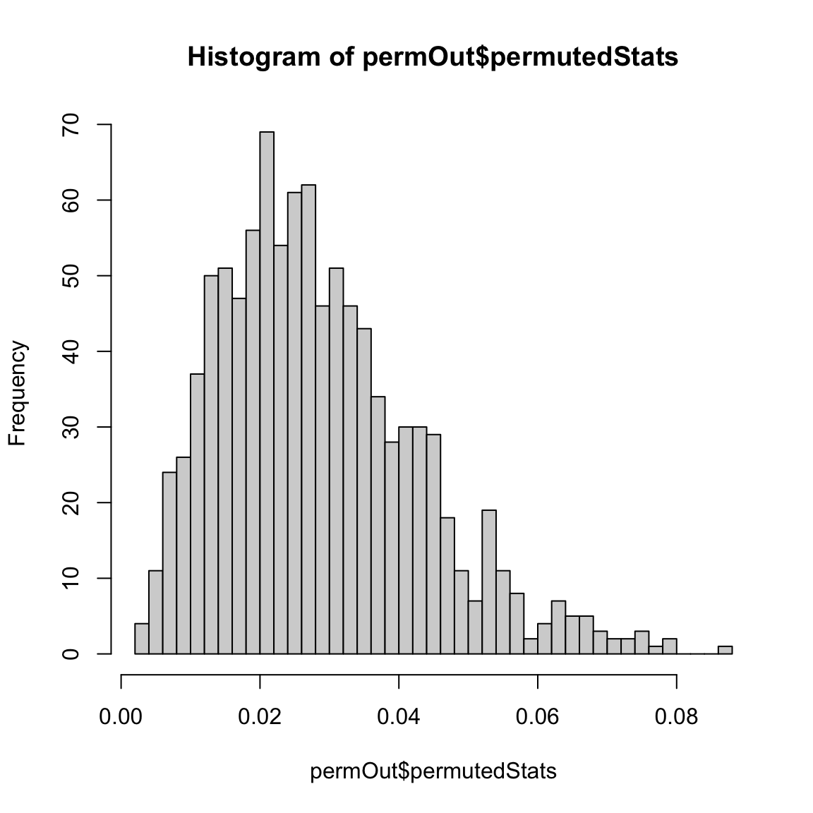
## $p.value
## [1] 0
##
## $observedStat
## [1] 0.7265596
Notice that we could also use the \(F\) statistic from before too (here we overlay the null distribution of the \(F\) statistic from the parametric model for comparison),
n <- nrow(body)
p <- ncol(body) - 1
permOutF <- permutationLM(body$BODYFAT, data = body[,
    -1], n.repetitions = 1000, STAT = function(lmFit) {
    summary(lmFit)$fstatistic["value"]
})
hist(permOutF$permutedStats, freq = FALSE, breaks = 50)
curve(df(x, df1 = p, df2 = n - p - 1), add = TRUE,
    main = paste("F(", p, ",", n - p - 1, ") distribution"))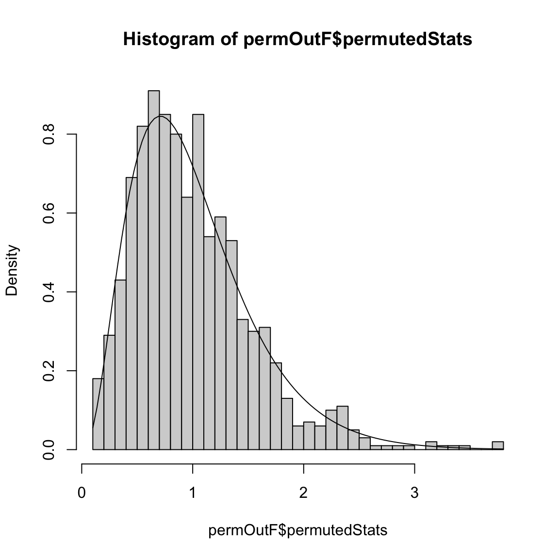
## $p.value
## [1] 0
##
## $observedStat
##    value
## 92.61904
6.6.3 Individual Variable Importance
We can also ask about individual variable, \(\beta_j\). This is a problem that we have discussed in the setting of simple regression, where we are interested in inference regarding the parameter \(\beta_j\), either with confidence intervals of \(\beta_j\) or the null hypothesis: \[H_0: \beta_j=0\]
In order to perform inference for \(\beta_j\), we have two possibilities of how to perform inference, like in simple regression: bootstrap CI and the parametric model.
6.6.3.1 Bootstrap for CI of \(\hat{\beta}_j\)
Performing the bootstrap to get CI for \(\hat{\beta}_j\) in multiple regression is the exact same procedure as in simple regression.
Specifically, we still bootstrap pairs \((y_i,x_i)\) and each time recalculate the linear model. For each \(\beta_j\), we will have a distribution of \(\hat{\beta}_j^*\) for which we can perform confidence intervals.
We can even use the same function as we used in the simple regression setting with little changed.
bootstrapLM <- function(y, x, repetitions, confidence.level = 0.95) {
    stat.obs <- coef(lm(y ~ ., data = x))
    bootFun <- function() {
        sampled <- sample(1:length(y), size = length(y),
            replace = TRUE)
        coef(lm(y[sampled] ~ ., data = x[sampled, ]))
    }
    stat.boot <- replicate(repetitions, bootFun())
    level <- 1 - confidence.level
    confidence.interval <- apply(stat.boot, 1, quantile,
        probs = c(level/2, 1 - level/2))
    return(list(confidence.interval = cbind(lower = confidence.interval[1,
        ], estimate = stat.obs, upper = confidence.interval[2,
        ]), bootStats = stat.boot))
}## lower estimate upper
## (Intercept) -75.68776383 -3.747573e+01 -3.84419402
## AGE -0.03722018 1.201695e-02 0.06645578
## WEIGHT -0.24629552 -1.392006e-01 -0.02076377
## HEIGHT -0.41327145 -1.028485e-01 0.28042319
## CHEST -0.25876131 -8.311678e-04 0.20995486
## ABDOMEN 0.81115069 9.684620e-01 1.13081481
## HIP -0.46808557 -1.833599e-01 0.10637834
## THIGH 0.02272414 2.857227e-01 0.56054626require(gplots)
with(bodyBoot, plotCI(confidence.interval[-1, "estimate"],
ui = confidence.interval[-1, "upper"], li = confidence.interval[-1,
"lower"], xaxt = "n"))
axis(side = 1, at = 1:(nrow(bodyBoot$conf) - 1), rownames(bodyBoot$conf)[-1])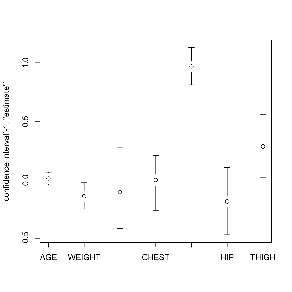
Note, that unless I scale the variables, I can’t directly interpret the size of the \(\beta_j\) as its importance (see commentary above under interpretation).
Assumptions of the Bootstrap
Recall that the bootstrap has assumptions, two important ones being that we have independent observations and the other being that we can reasonably estimate \(F\) with \(\hat{F}\). However, the distribution \(F\) we need to estimate is not the distribution of an individual a single variable, but the entire joint distributions of all the variables. This gets to be a harder and harder task for larger numbers of variables (i.e. for larger \(p\)).
In particular, when using the bootstrap in multiple regression, it will not perform well if \(p\) is large relative to \(n\).56 In general you want the ratio \(p/n\) to be small (like less than 0.1); otherwise the bootstrap can give very poor CI.57
## Ratio of p/n in body fat: 0.031746036.6.3.2 Parametric models
Again, our inference on \(\beta_j\) will look very similar to simple regression. Using our parametric assumptions about the distribution of the errors will mean that each \(\hat{\beta}_j\) is normally distributed 58 \[\hat{\beta}_j \sim N(\beta_j, \nu^2_j)\] where \[\nu^2_j=\ell(X)\sigma^2\] (\(\ell(X)\) is a linear combination of all of the observed explanatory variables, given in the matrix \(X\)).59
Using this, we create t-statistics for each \(\beta_j\) by standardizing \(\hat{\beta}_j\)
\[T_j=\frac{\hat{\beta_j}}{\sqrt{\hat{var}(\hat{\beta_j})}}\]
Just like the t-test, \(T_j\) should be normally distributed60
This is exactly what lm gives us:
##                  Estimate  Std. Error      t value     Pr(>|t|)
## (Intercept) -3.747573e+01 14.49480190 -2.585460204 1.030609e-02
## AGE          1.201695e-02  0.02933802  0.409603415 6.824562e-01
## WEIGHT      -1.392006e-01  0.04508534 -3.087490946 2.251838e-03
## HEIGHT      -1.028485e-01  0.09787473 -1.050817489 2.943820e-01
## CHEST       -8.311678e-04  0.09988554 -0.008321202 9.933675e-01
## ABDOMEN      9.684620e-01  0.08530838 11.352484708 2.920768e-24
## HIP         -1.833599e-01  0.14475772 -1.266667813 2.064819e-01
## THIGH        2.857227e-01  0.13618546  2.098041564 3.693019e-02
Correlation of estimates
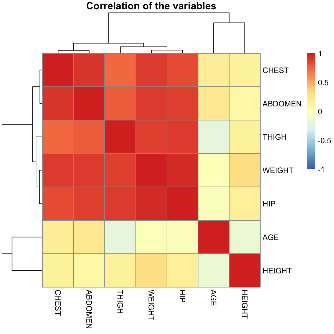
The estimated \(\hat{\beta}_j\) are themselves correlated with each other, unless the \(x^{j}\) and \(x^{k}\) variables are uncorrelated.
library(pheatmap)
pheatmap(summary(ft, correlation = TRUE)$corr[-1, -1],
    breaks = seq(-1, 1, length = 100), main = "Correlation of the estimated coefficients")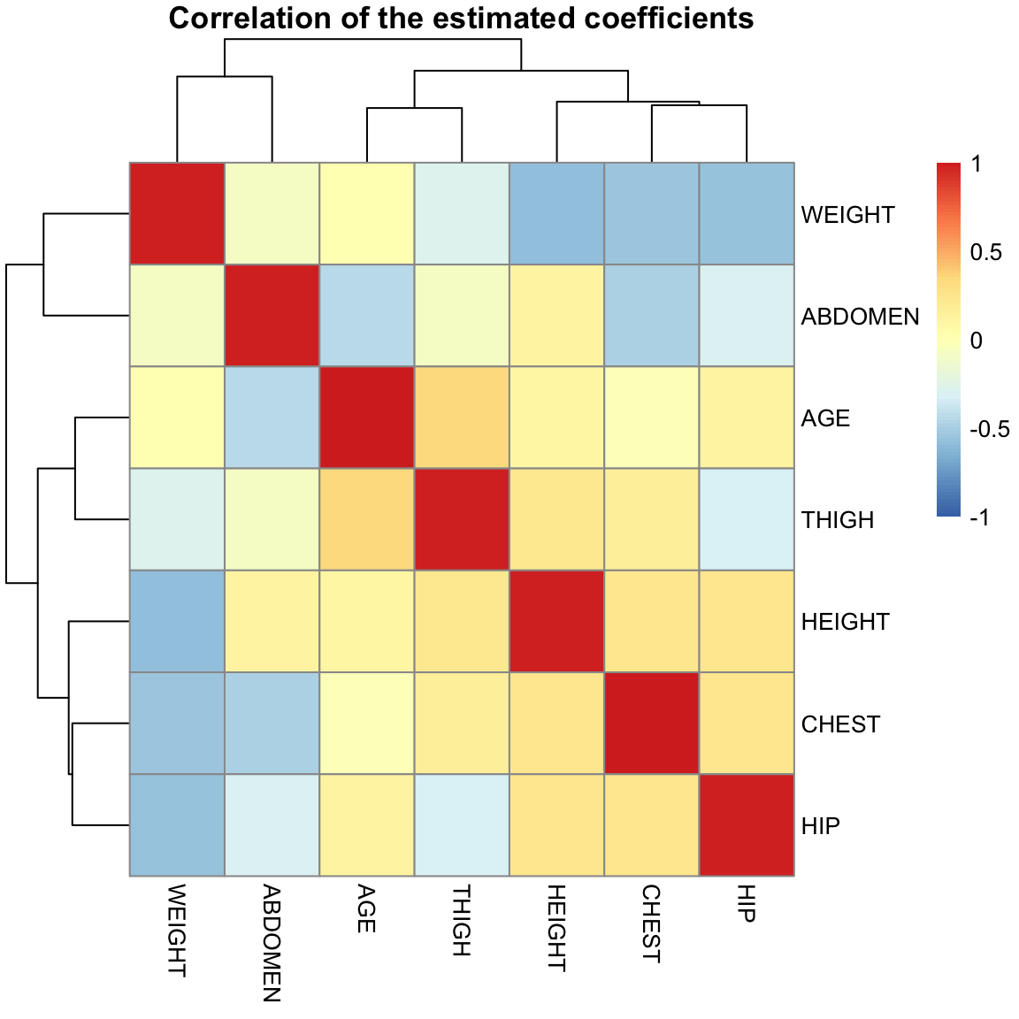
6.6.4 Inference on \(\hat{y}(x)\)
We can also create confidence intervals on the prediction given by the model, \(\hat{y}(x)\). For example, suppose now that we are asked to predict the bodyfat percentage of an individual who has a particular set of variables \(x_0\). Then the same logic in simple regression follows here.
There are two intervals associated with prediction:
- Confidence intervals for the average response, i.e. bodyfat percentage for all individuals who have the values \(x_0\). The average (or expected values) at \(x_0\) is \[E(y(x_0))=\beta_0+\beta_1 x_0^{(1)}+\ldots+\beta_p x_0^{(p)}.\] and so we estimate it using our estimates of \(\beta_j\), getting \(\hat{y}(x_0)\).
Then our \(1-\alpha\) confidence interval will be61 \[\hat{y}(x_0) \pm t_{\alpha_2} \sqrt{\hat{var}(\hat{y}(x_0) )}\]
- Confidence intervals for a particular individual (prediction interval). If we knew \(\beta\) completely, we still wouldn’t know the value of the particular individual. But if we knew \(\beta\), we know that our parametric model says that all individuals with the same \(x_0\) values are normally distributed as \[N(\beta_0+\beta_1 x_0^{(1)}+\ldots+\beta_p x_0^{(p)}, \sigma^2) \]
So we could give an interval that we would expect 95% confidence that such an individual would be in, how?
We don’t know \(\beta\), so actually we have to estimate both parts of this, \[\hat{y}(x_0)+\pm 1.96 \sqrt{\hat{\sigma}^2+ \hat{var}(\hat{y}(x_0) )}\]
Both of these intervals are obtained in R via the predict function.
x0 = data.frame(AGE = 30, WEIGHT = 180, HEIGHT = 70,
    CHEST = 95, ABDOMEN = 90, HIP = 100, THIGH = 60)
predict(ft, x0, interval = "confidence")
## fit lwr upr
## 1 16.51927 15.20692 17.83162## fit lwr upr
## 1 16.51927 7.678715 25.35983Note that the prediction interval is much wider compared to the confidence interval for average response.
% % ## Regression Diagnostics
Our next topic in multiple regression is regression diagnostics. The inference procedures that we talked about work under the assumptions of the linear regression model. If these assumptions are violated, then our hypothesis tests, standard errors and confidence intervals will be violated. Regression diagnostics enable us to diagnose if the model assumptions are violated or not.
The key assumptions we can check for in the regression model are:
- Linearity: the mean of the \(y\) is linearly related to the explanatory variables.
- Homoscedasticity: the errors have the same variance.
- Normality: the errors have the normal distribution.
- All the observations obey the same model (i.e., there are no outliers or exceptional observations).
These are particularly problems for the parametric model; the bootstrap will be relatively robust to these assumptions, but violations of these assumptions can cause the inference to be less powerful – i.e. harder to detect interesting signal.
These above assumptions can be checked by essentially looking at the residuals:
- Linearity: The residuals represent what is left in the response variable after the linear effects of the explanatory variables are taken out. So if there is a non-linear relationship between the response and one or more of the explanatory variables, the residuals will be related non-linearly to the explanatory variables. This can be detected by plotting the residuals against the explanatory variables. It is also common to plot the residuals against the fitted values. Note that one can also detect non-linearity by simply plotting the response against each of the explanatory variables.
- Homoscedasticity: Heteroscedasticity can be checked again by plotting the residuals against the explanatory variables and the fitted values. It is common here to plot the absolute values of the residuals or the square root of the absolute values of the residuals.
- Normality: Detected by the normal Q-Q plot of the residuals.
- Outliers: The concern with outliers is that they could be effecting the fit. There are three measurements we could use to consider whether a point is an outlier
- Size of the residuals (\(r_i\)) – diagnostics often use standardized residuals to make them more comparable between different observations62
- Leverage – a measure of how far the vector of explanatory variables of an observation are from the rest, and on average are expected to be about \(p/n\).
- Cook’s Distance – how much the coefficients \(\hat{\beta}\) will change if you leave out observation \(i\), which basically combines the residual and the leverage of a point.
Outliers typically will have either large (in absolute value) residuals and/or large leverage.
Consider the bodyfat dataset. A simple way for doing some of the standard regression diagnostics is to use the plot
command as applied to the linear model fit:
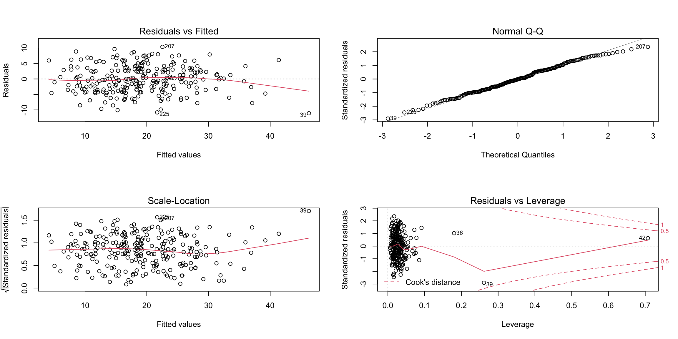
Let’s go through these plots and what we can look for in these plots. There can sometimes be multiple issues that we can detect in a single plot.
Independence
Note that the most important assumption is independence. Violations of independence will cause problems for every inference procedure we have looked at, including the resampling procedures, and the problems such a violation will cause for your inference will be even worse than the problems listed above. Unfortunately, violations of independence are difficult to check for in a generic problem. If you suspect a certain kind of dependence, e.g. due to time or geographical proximity, there are special tools that can be used to check for that. But if you don’t have a candidate for what might be the source of the dependence, the only way to know there is no dependence is to have close control over how the data was collected.
6.6.5 Residuals vs. Fitted Plot
The first plot is the residuals plotted against the fitted values. The points should look like a random scatter with no discernible pattern. We are often looking for two possible violations:
- Non-linear relationship to response, detected by a pattern in the mean of the residuals. Recall that the correlation between \(\hat{y}\) and the residuals must be numerically zero – but that doesn’t mean that there can’t be non-linear relationships.
- Heteroscedasticity – a pattern in the variability of the residuals, for example higher variance in observations with large fitted values.
Let us now look at some simulation examples in the simple setting of a single predictor to demonstrate these phenomena.
Example: Non-linearity
In the next example, the response is related non-linearly to \(x\).
n = 200
xx1 = 3 + 4 * abs(rnorm(n))
yy1 = -2 + 0.5 * xx1^(1.85) + rnorm(n)
m1 = lm(yy1 ~ xx1)
par(mfrow = c(1, 2))
plot(yy1 ~ xx1)
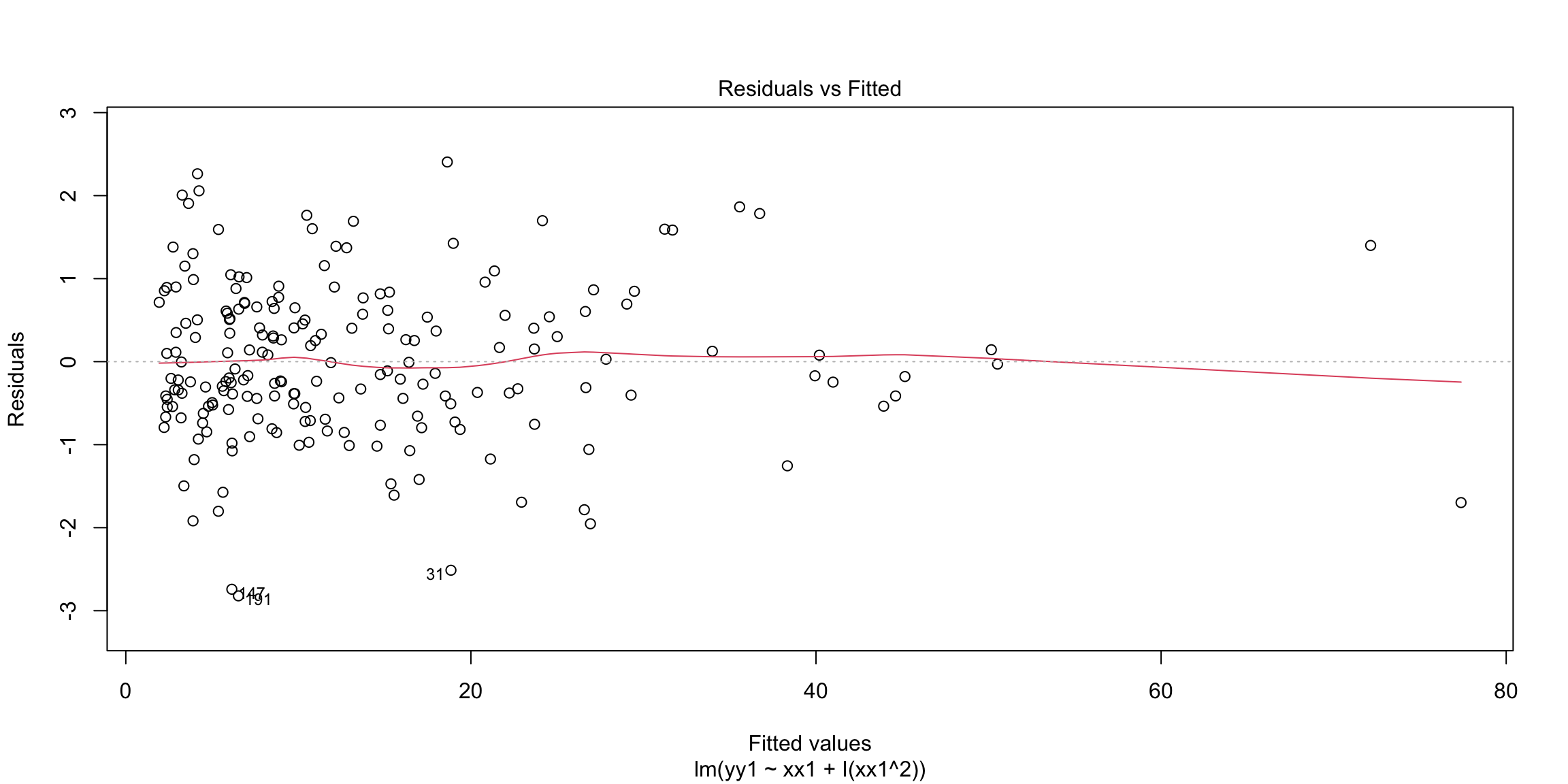
plot(m1, which = 1)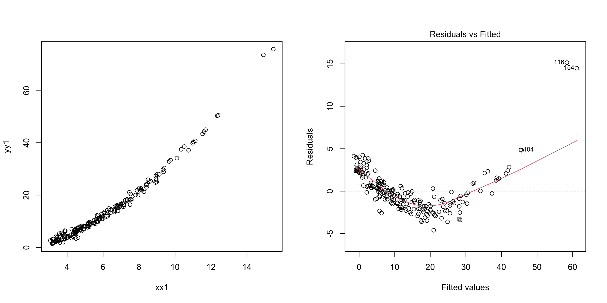 Non-linearity is fixed by adding non-linear functions of explanatory
variables as additional explanatory variables. In this example, for
instance, we can add \(x^2\) as an additional explanatory variable.
Non-linearity is fixed by adding non-linear functions of explanatory
variables as additional explanatory variables. In this example, for
instance, we can add \(x^2\) as an additional explanatory variable.
Example: Heteroscedasticity
Next let us consider an example involving heterscedasticity (unequal variance).
set.seed(478912)
n = 200
xx2 = 3 + 4 * abs(rnorm(n))
yy2 = -2 + 5 * xx2 + 0.5 * (xx2^(1.5)) * rnorm(n)
m2 = lm(yy2 ~ xx2)
par(mfrow = c(1, 2))
plot(yy2 ~ xx2)
plot(m2, which = 1)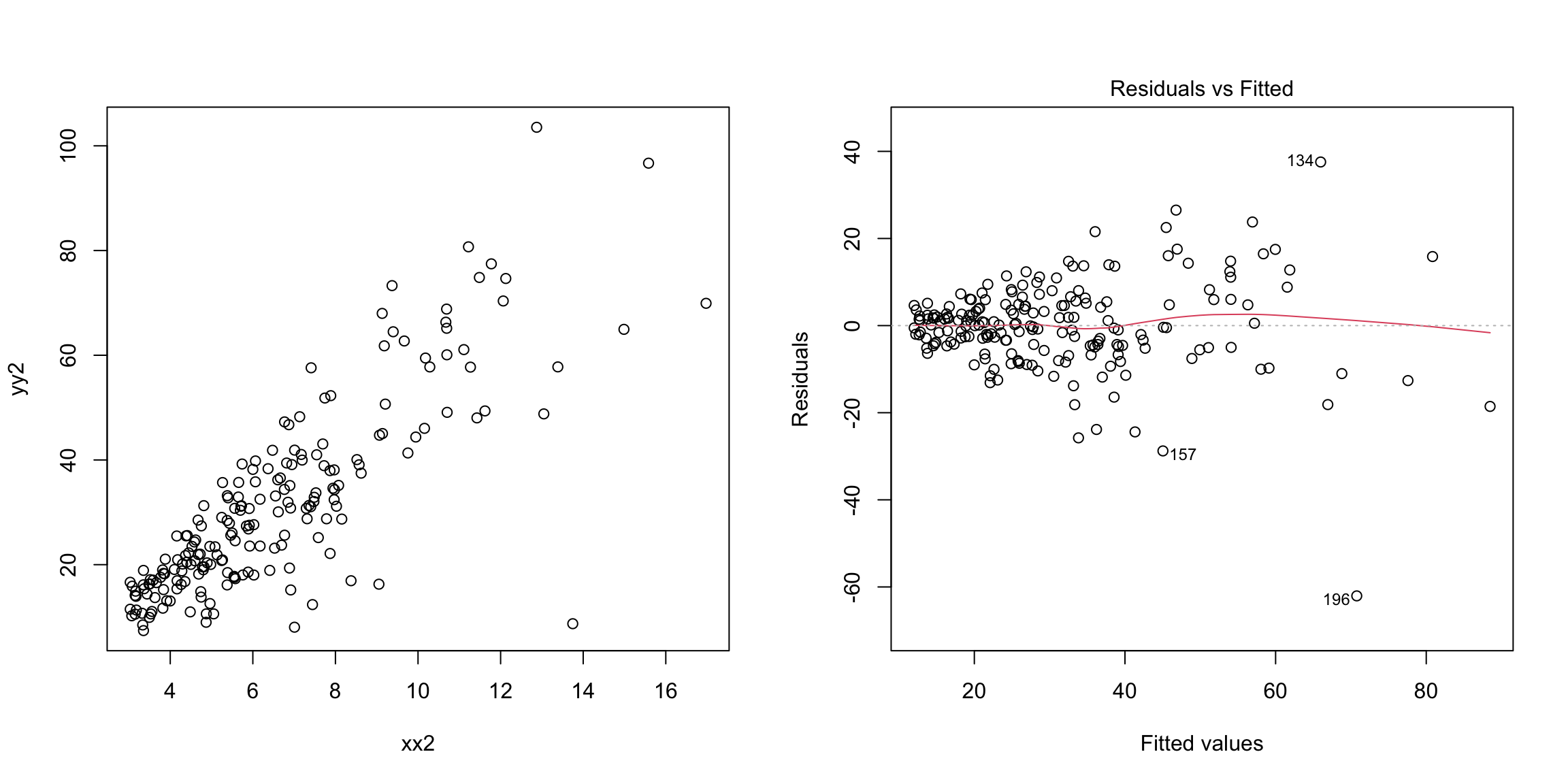 Notice that even with a single variable, it is easier to see the difference in variability with the residuals than in plotting \(y\) versus \(x\) (in the plot of \(y\) versus \(x\), the fact that \(y\) is growing with \(x\) makes it harder to be sure).
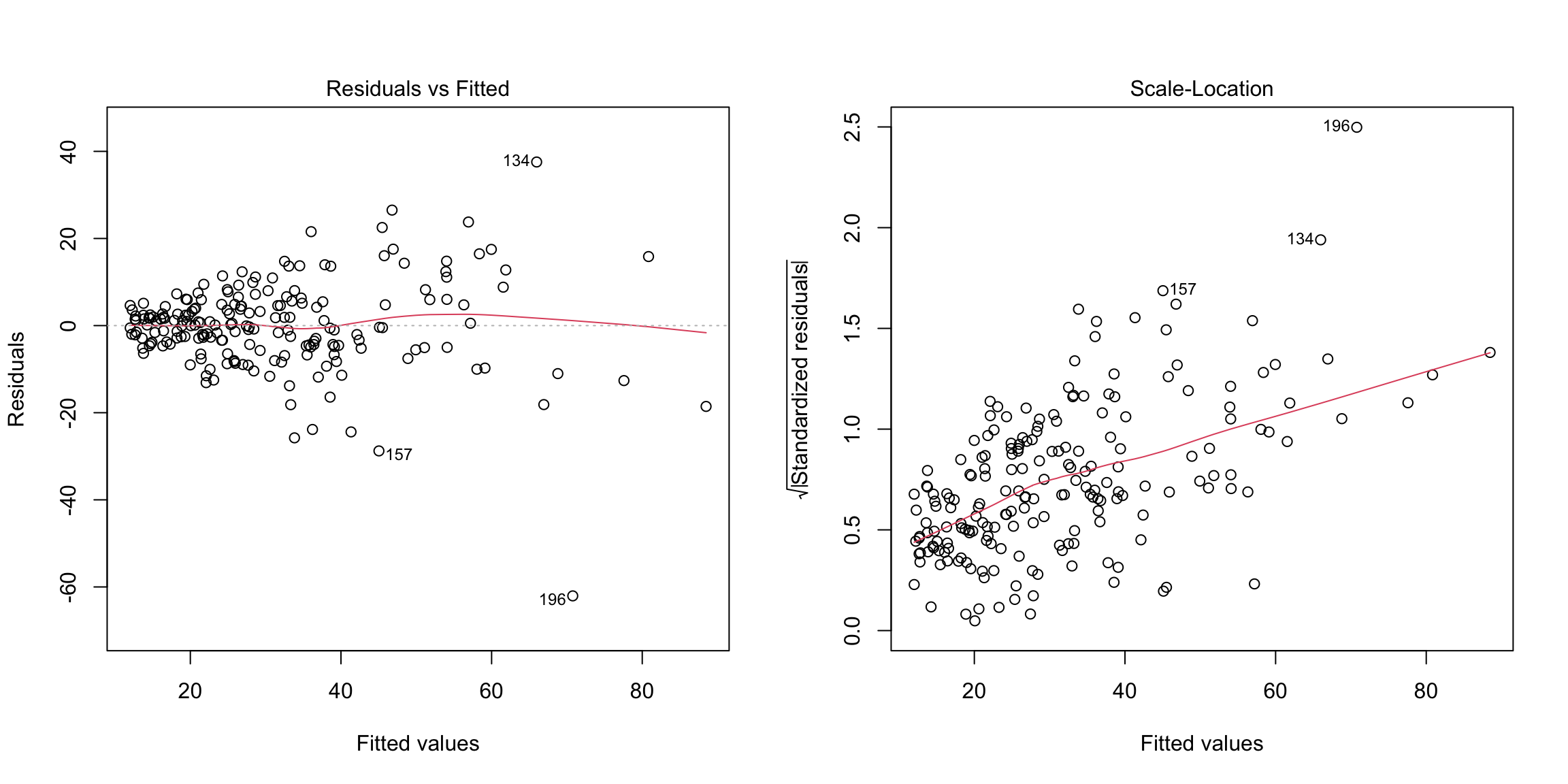
Heteroscedasticity is a little tricky to handle in general. Heteroscedasiticity can sometimes be fixed by applying a transformation to the response variable (\(y\)) before fitting the regression. For example, if all the response values are positive, taking the logarithm or square root of the response variable is a common solution.
The Scale-Location plot (which is one of the default plots of plot) is also useful for detecting heteroscedasiticity. It plots the square
root of the absolute value of the residuals (actually standardized
residuals but these are similar to the residuals) against the fitted
values. Any increasing or decreasing pattern in this plot indicates
heteroscedasticity. Here is that plot on the simulated data that has increasing variance:
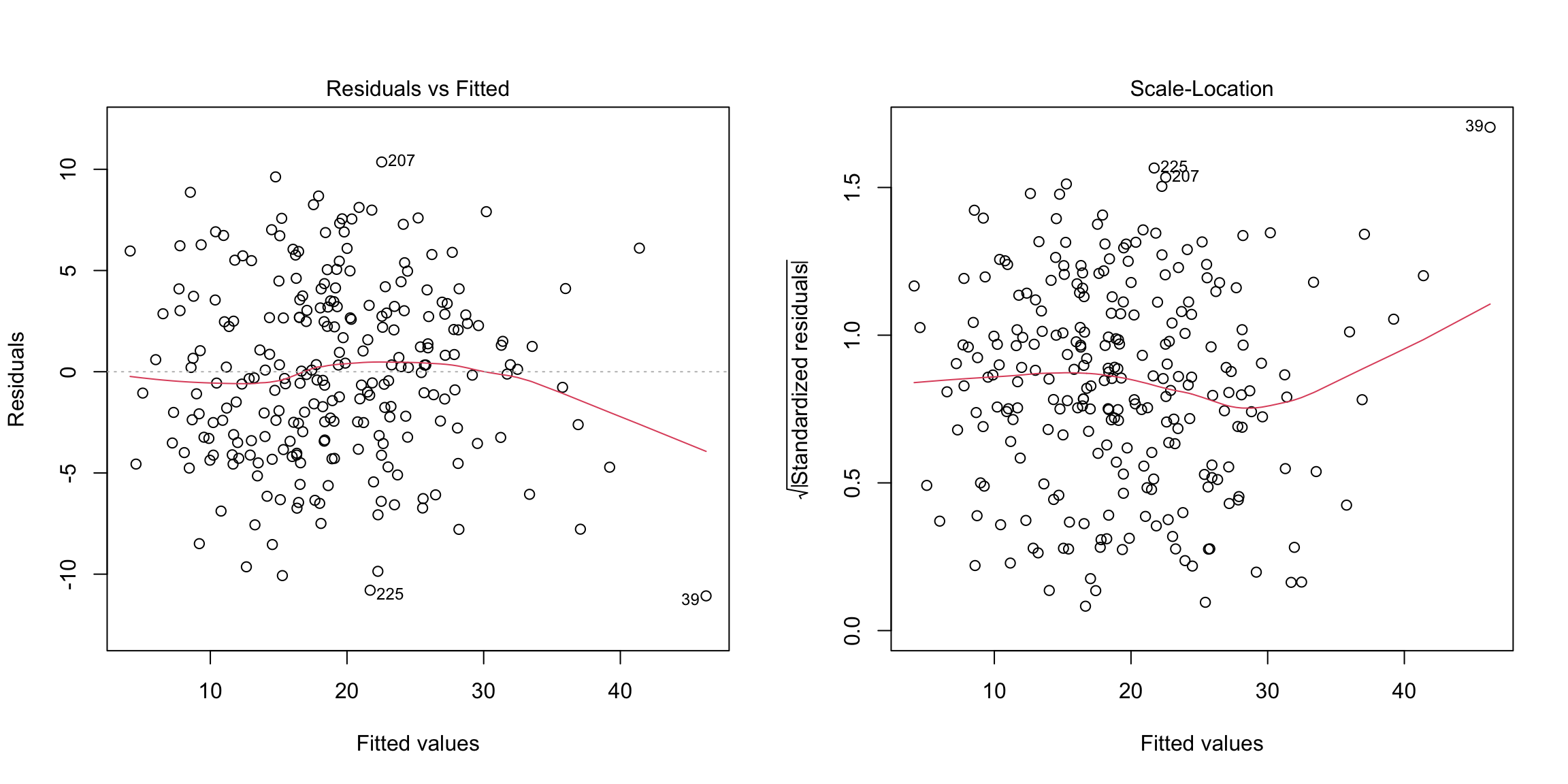
Back to data
We don’t see any obvious pattern in the fitted versus residual plot.
We do the same plot from our bike regression from above:
md1 = lm(casual ~ atemp + workingday + weathersit,
    data = bike)
par(mfrow = c(1, 2))
plot(md1, which = c(1, 3))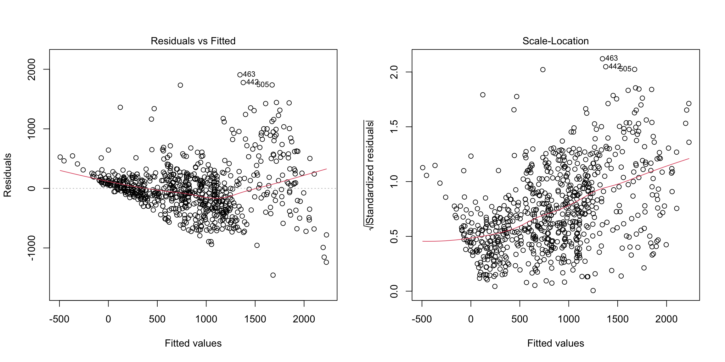
Here we see serious heteroskedasticity, where there is more variability in our residuals for larger fitted values than for smaller ones. There’s also possibly signs that our residuals have a pattern to them (not centered at zero), possibly indicating that our linear fit is not appropriate.
The response here is counts (number of casual users) and it is common to transform such data. Here we show the fitted/residual plot after transforming the response by the log and square-root:
mdLog = lm(log(casual) ~ atemp + workingday + weathersit,
    data = bike)
mdSqrt = lm(sqrt(casual) ~ atemp + workingday + weathersit,
    data = bike)
par(mfrow = c(2, 2))
plot(mdLog, which = 1, main = "Log")
plot(mdSqrt, which = 1, main = "Sqrt")
plot(mdLog, which = 3, main = "Log")
plot(mdSqrt, which = 3, main = "Sqrt")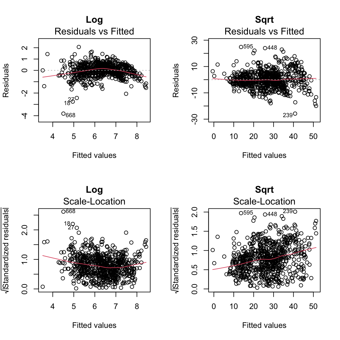
Why plot against \(\hat{y}\)?
If we think there is a non linear relationship, shouldn’t we plot against the individual \(x^{(j)}\) variables? We certainly can! Just like with \(\hat{y}\), each \(x^{(j)}\) is uncorrelated with the residuals, but there can be non-linear relationships that show up. Basically any plot we do of the residuals should look like a random cloud of points with no pattern, including against the explanatory variables.
Plotting against the individual \(x^{(j)}\) can help to determine which variables have a non-linear relationship, and can help in determining an alternative model. Of course this is only feasible with a relatively small number of variables.
One reason that \(\hat{y}\) is our default plot is that 1) there are often too many variables to plot against easily; and 2) there are many common examples where the variance changes as a function of the size of the response, e.g. more variance for larger \(y\) values.
6.6.6 QQ-Plot
The second plot is the normal Q-Q plot of the standardized residuals. If the normal assumption holds, then the points should be along the line here.
library(MASS)
par(mfrow = c(1, 2))
hist(stdres(ft), freq = FALSE, breaks = 10, xlim = c(-3.5,
    3.5))
curve(dnorm, add = TRUE)
plot(ft, which = 2)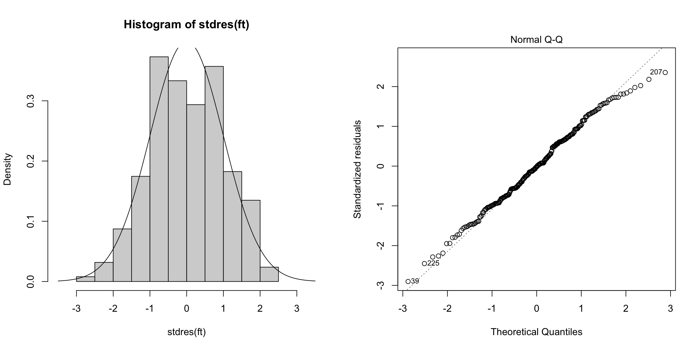
A QQ-plot is based on the idea that every point in your dataset is a quantile. Specifically, if you have data \(x_1,\ldots,x_n\) and you assume they are all in order, then the probability of finding a data point less than or equal to \(x_1\) is \(1/n\) (assuming there are no ties). So \(x_1\) is the \(1/n\) quantile of the observed data distribution. \(x_2\) is the \(2/n\) quantile, and so forth.63
## 0.3968254%
##  -2.453687
Under our assumption of normality, then we also know what the \(1/n\) quantile should be based on qnorm (the standardized residuals are such that we expect them to be \(N(0,1)\))
## [1] -2.654759The idea with QQ-plots is that we can do this for all of the data, and compare whether our data has quantiles that match what we would expect for a normal distribution.
Here are some examples of QQ-plots for some simulated data, to give you a sense of how QQ-plots correspond to distributional properties:
par(mfrow = c(4, 2), cex = 2)
n <- 500
qqlim <- c(-4, 4)
set.seed(302)
x <- rnorm(n)
x <- scale(x, scale = TRUE)
hist(x, freq = FALSE, breaks = 10, xlim = c(-4, 4),
    main = "Normal Data")
curve(dnorm, add = TRUE)
qqnorm(x, xlim = qqlim, ylim = qqlim)
qqline(x)
x <- rt(n, df = 3)
x <- scale(x, scale = TRUE)
hist(x, freq = FALSE, breaks = 30, xlim = c(-4, 4),
    main = "Heavy Tailed")
curve(dnorm, add = TRUE)
qqnorm(x, xlim = qqlim, ylim = qqlim)
qqline(x)
x <- rnorm(n, 0, 1)
x <- scale(sign(x) * abs(x)^{
    3/4
}, scale = TRUE)
hist(x, freq = FALSE, breaks = 10, xlim = c(-4, 4),
    main = "Light Tailed")
curve(dnorm, add = TRUE)
qqnorm(x, xlim = qqlim, ylim = qqlim)
qqline(x)
x <- rgamma(n, 5, 1)
x <- scale(x, scale = TRUE)
hist(x, freq = FALSE, breaks = 10, xlim = c(-4, 4),
    main = "Skewed")
curve(dnorm, add = TRUE)
qqnorm(x, xlim = qqlim, ylim = qqlim)
qqline(x)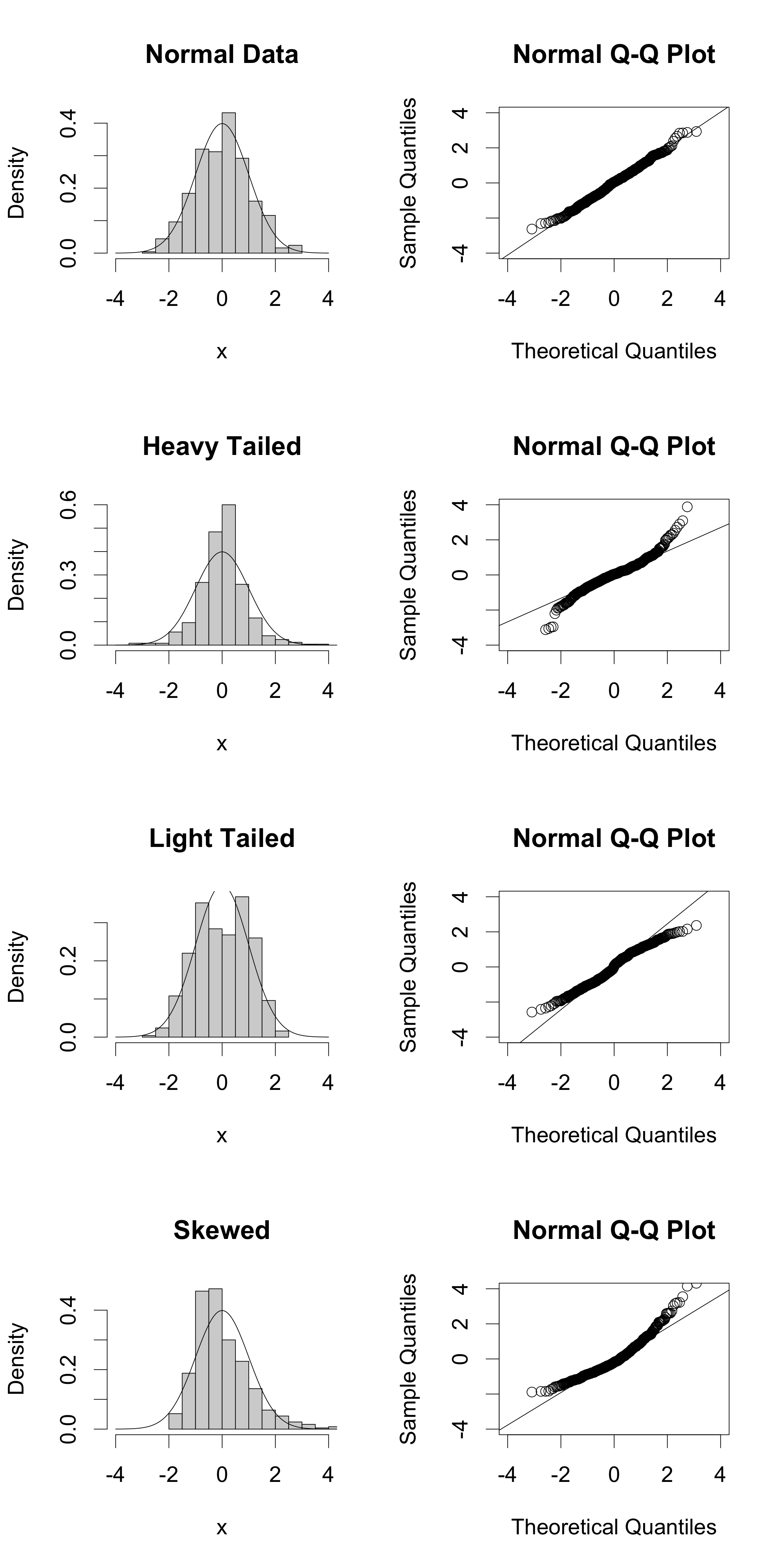
Back to body fat data
There are some signs in the right tail that the residuals are a little off normal.
Would you say that they are heavy or light tailed?
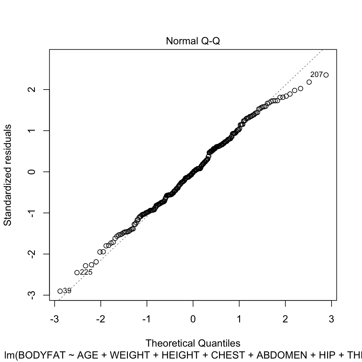
Looking at the bike model, we see the QQ plot shows serious problems in the residuals as well. We see that taking a transformation of the response not only helped with the heteroskedasticity, but also makes the residuals look closer to normal. This is not uncommon, that what helps create more constant variance can help the distributional assumptions as well.
par(mfrow = c(2, 2))
plot(md1, which = 2, main = "Original (counts)")
plot(mdLog, which = 2, main = "Log")
plot(mdSqrt, which = 2, main = "Sqrt")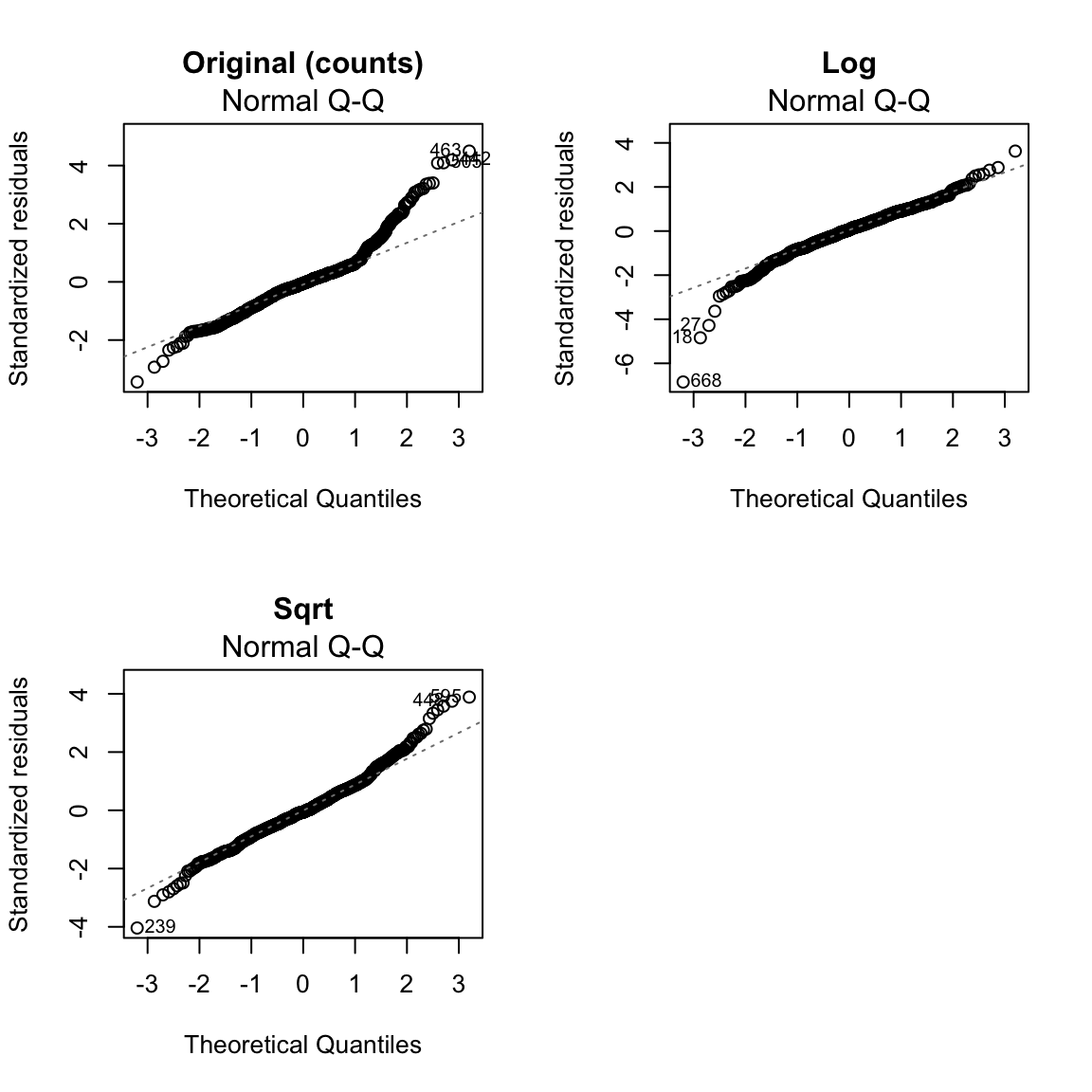
6.6.7 Detecting outliers
The final plots are used for detecting outliers and other exceptional observations. Large leverage or large residuals can indicate potential outliers, as does cooks distance, which is a combination of the two. The default plots give the index of potential outliers to help identify them.
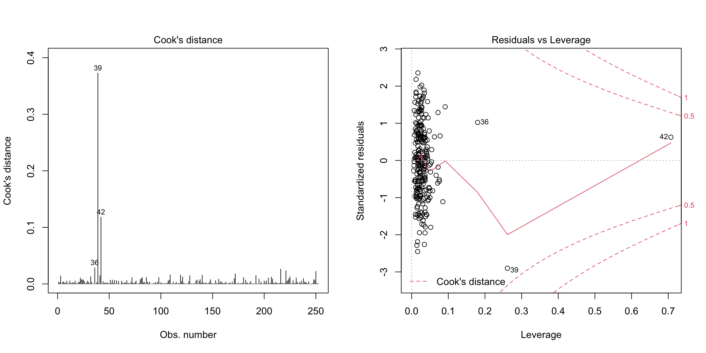
Three points flagged here are observations \(i=39, 42,36\). Let us look at these observations separately, as well as plot some our visualizations highlighting these points:
## High leverage points:## BODYFAT AGE WEIGHT HEIGHT CHEST ABDOMEN HIP THIGH
## 39 35.2 46 363.15 72.25 136.2 148.1 147.7 87.3
## 42 32.9 44 205.00 29.50 106.0 104.3 115.5 70.6
## 36 40.1 49 191.75 65.00 118.5 113.1 113.8 61.9## Mean of each variables:## BODYFAT AGE WEIGHT HEIGHT CHEST ABDOMEN HIP THIGH
## 19.15079 44.88492 178.92440 70.14881 100.82421 92.55595 99.90476 59.40595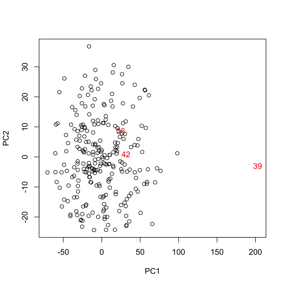
pairs(body, panel = function(x, y) {
    points(x[-whOut], y[-whOut])
    text(x[whOut], y[whOut], labels = whOut)
})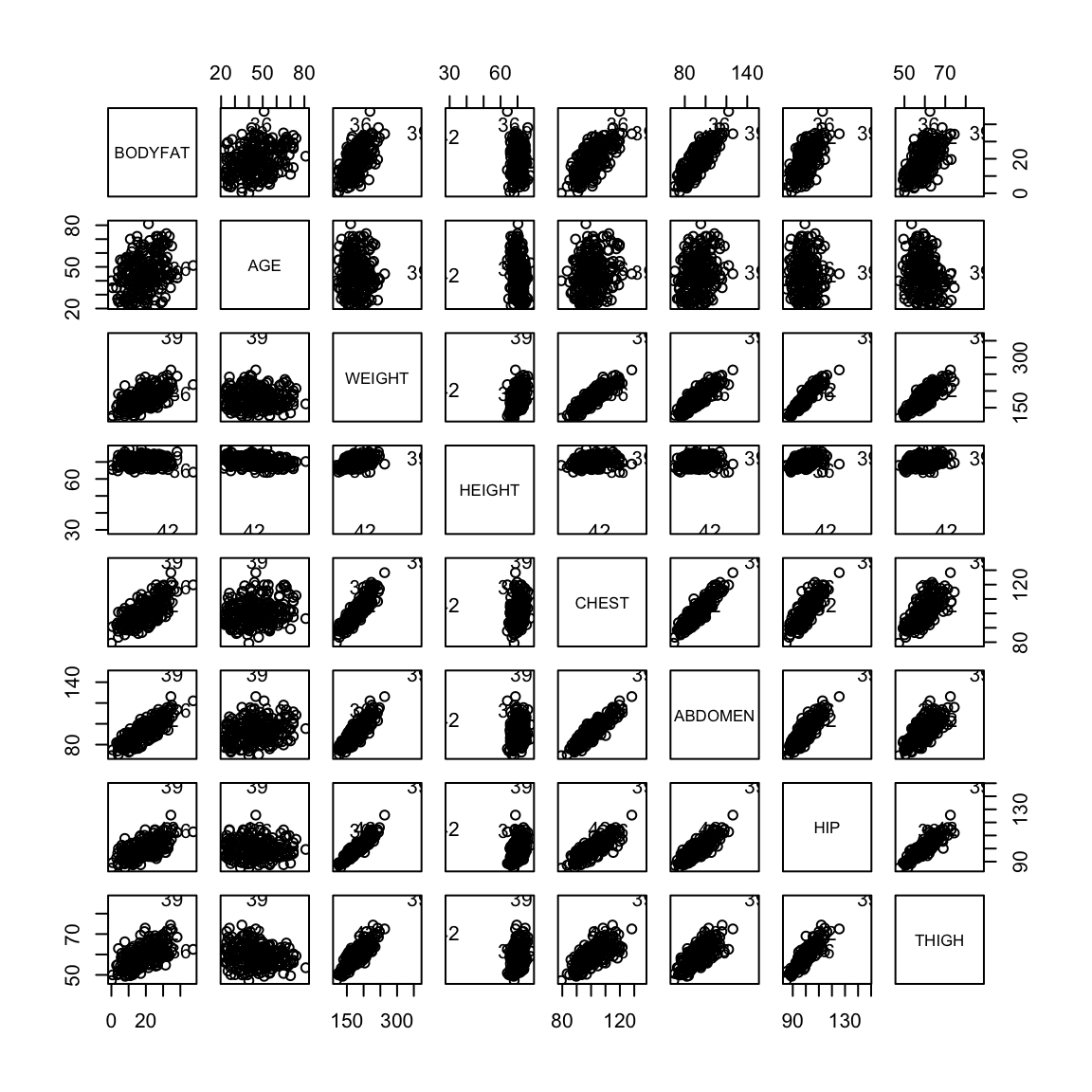
The observation 39 is certainly an outlier in many variables. Observation 42 seems to have an erroneous height recording. Observation 36 seems to have a high value for the response (percent bodyfat).
When outliers are detected, one can perform the regression analysis after dropping the outlying observations and evaluate their impact. After this, one needs to decide whether to report the analysis with the outliers or without them.
## Coefficients without outliers:## Estimate Std. Error t value Pr(>|t|)
## (Intercept) -22.902 20.297 -1.128 0.260
## AGE 0.021 0.029 0.717 0.474
## WEIGHT -0.074 0.059 -1.271 0.205
## HEIGHT -0.241 0.187 -1.288 0.199
## CHEST -0.121 0.113 -1.065 0.288
## ABDOMEN 0.945 0.088 10.709 0.000
## HIP -0.171 0.152 -1.124 0.262
## THIGH 0.223 0.141 1.584 0.114##
## Coefficients in Original Model:## Estimate Std. Error t value Pr(>|t|)
## (Intercept) -37.476 14.495 -2.585 0.010
## AGE 0.012 0.029 0.410 0.682
## WEIGHT -0.139 0.045 -3.087 0.002
## HEIGHT -0.103 0.098 -1.051 0.294
## CHEST -0.001 0.100 -0.008 0.993
## ABDOMEN 0.968 0.085 11.352 0.000
## HIP -0.183 0.145 -1.267 0.206
## THIGH 0.286 0.136 2.098 0.037We can see that WEIGHT and THIGH are no longer significant after removing these outlying points. We should note that removing observations reduces the power of all tests, so you may often see less significance if you remove many points (three is not really many!). But we can compare to removing three random points, and see that we don’t have major changes in our results:
## Coefficients without three random points:## Estimate Std. Error t value Pr(>|t|)
## (Intercept) -36.732 14.620 -2.513 0.013
## AGE 0.008 0.030 0.287 0.774
## WEIGHT -0.139 0.045 -3.070 0.002
## HEIGHT -0.108 0.098 -1.094 0.275
## CHEST 0.002 0.100 0.016 0.987
## ABDOMEN 0.972 0.086 11.351 0.000
## HIP -0.182 0.145 -1.249 0.213
## THIGH 0.266 0.136 1.953 0.0526.7 Variable Selection
Consider a regression problem with a response variable \(y\) and \(p\) explanatory variables \(x_1, \dots, x_p\). Should we just go ahead and fit a linear model to \(y\) with all the \(p\) explanatory variables or should we throw out some unnecessary explanatory variables and then fit a linear model for \(y\) based on the remaining variables? One often does the latter in practice. The process of selecting important explanatory variables to include in a regression model is called variable selection. The following are reasons for performing variable selection:
- Removing unnecessary variables results in a simpler model. Simpler models are always preferred to complicated models.
- Unnecessary explanatory variables will add noise to the estimation of quantities that we are interested in.
- Collinearity (i.e. strong linear relationships in the variables) is a problem with having too many variables trying to do the same job.
- We can save time and/or money by not measuring redundant explanatory variables.
Several common, interrelated strategies for asking this question
- Hypothesis testing on variables or submodels
- Stepwise regression based on \(p\)-values
- Criteria based Variable Selection
We shall illustrate variable selection procedures using the following
dataset (which is available in R from the faraway package). This small dataset gives information about drivers and the seat position that they choose, with the idea of trying to predict a seat position from information regarding the driver (age, weight, height,…).
We can see that the variables are highly correlated with each other, and no variables are significant. However, the overall \(p\)-value reported for the \(F\)-statistic in the summary is almost zero (this is an example of how you might actually find the \(F\) statistic useful, in that it provides a check that even though no single variable is significant, the variables jointly do fit the data well )
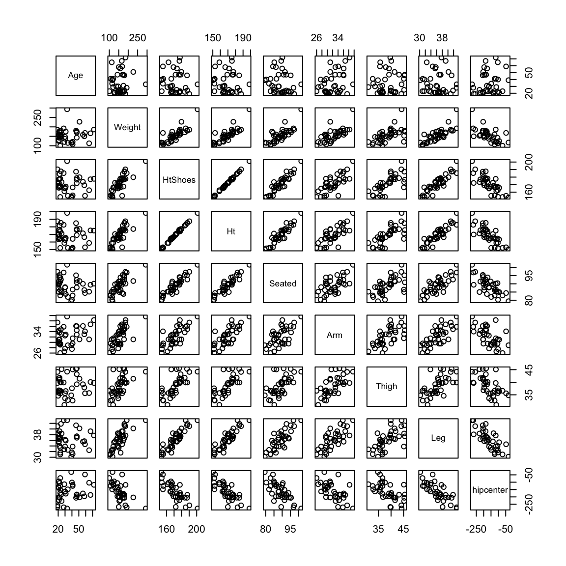
##
## Call:
## lm(formula = hipcenter ~ ., data = seatpos)
##
## Residuals:
##     Min      1Q  Median      3Q     Max
## -73.827 -22.833  -3.678  25.017  62.337
##
## Coefficients:
##              Estimate Std. Error t value Pr(>|t|)
## (Intercept) 436.43213  166.57162   2.620   0.0138 *
## Age           0.77572    0.57033   1.360   0.1843
## Weight        0.02631    0.33097   0.080   0.9372
## HtShoes      -2.69241    9.75304  -0.276   0.7845
## Ht            0.60134   10.12987   0.059   0.9531
## Seated        0.53375    3.76189   0.142   0.8882
## Arm          -1.32807    3.90020  -0.341   0.7359
## Thigh        -1.14312    2.66002  -0.430   0.6706
## Leg          -6.43905    4.71386  -1.366   0.1824
## ---
## Signif. codes:  0 '***' 0.001 '**' 0.01 '*' 0.05 '.' 0.1 ' ' 1
##
## Residual standard error: 37.72 on 29 degrees of freedom
## Multiple R-squared:  0.6866, Adjusted R-squared:  0.6001
## F-statistic:  7.94 on 8 and 29 DF,  p-value: 1.306e-05
6.7.1 Submodels and Hypothesis testing
We already saw that we can evaluate if we need any of the variables by setting up two models
Model 0: No variables, just predict \(\bar{y}\) for all observations
Model 1: Our linear model with all the variables
Then we compare the RSS from these two models with the F-statistic, \[F=\frac{(RSS_0-RSS_1)/p}{RSS_1/(n-p-1)}\] which the null hypothesis that these two models are equivalent (and assuming our parametric model) has a \(F\) distribution \[H_0: F \sim F(p, n-p-1)\]
We can expand this framework to compare any submodel to the full model, where a submodel means using only a specific subset of the \(p\) parameters. For example, can we use a model with only ABDOMEN, AGE, and WEIGHT?
For convenience lets say we number our variables so we have the first \(q\) variables are our submodel (\(q=3\) in our example). Then we now have two models:
Model 0: Just the first \(q\) variables (and the intercept) Model 1: Our linear model with all the \(p\) variables
We can do the same as before and calculate our \(RSS\) for each model and compare them. We can get a \(F\) statistic, \[F=\frac{(RSS_0-RSS_1)/(p-q)}{RSS_1/(n-p-1)}\] and under the null hypothesis that the two models are equivalent, \[H_0: F \sim F(p-q, n-p-1)\]
What does it mean if I get a non-significant result?
We can do this in R by fitting our two models, and running on the function anova on both models:
## Analysis of Variance Table
##
## Model 1: BODYFAT ~ ABDOMEN + AGE + WEIGHT
## Model 2: BODYFAT ~ AGE + WEIGHT + HEIGHT + CHEST + ABDOMEN + HIP + THIGH
##   Res.Df    RSS Df Sum of Sq      F Pr(>F)
## 1    248 4941.3
## 2    244 4806.8  4     134.5 1.7069 0.1491
What conclusion do we draw?
F-test is only valid for comparing submodels It is important to realize that the \(F\) test described here is only valid for comparing submodels, i.e. the smaller model has to be a set of variables that are a subset of the full model. You can’t compare disjoint sets of variables with an \(F\)-test.
Single variable: test for \(\beta_j\):
We could set up the following two models:
Model 0: All of the variables except for \(\beta_j\) Model 1: Our linear model with all the \(p\) variables
This is equivalent to \[H_0: \beta_j=0\]
How would you calculate the \(F\) statistic and null distribution of the \(F\) Statistic?
Here we run that leaving out just HEIGHT:
modNoHEIGHT <- lm(BODYFAT ~ ABDOMEN + AGE + WEIGHT +
    CHEST + HIP + THIGH, data = body)
anova(modNoHEIGHT, ft)
## Analysis of Variance Table
##
## Model 1: BODYFAT ~ ABDOMEN + AGE + WEIGHT + CHEST + HIP + THIGH
## Model 2: BODYFAT ~ AGE + WEIGHT + HEIGHT + CHEST + ABDOMEN + HIP + THIGH
## Res.Df RSS Df Sum of Sq F Pr(>F)
## 1 245 4828.6
## 2 244 4806.8 1 21.753 1.1042 0.2944In fact if we compare that with the inference from our standard t-test of \(\beta_j=0\), we see we get the same answer
##
## Call:
## lm(formula = BODYFAT ~ AGE + WEIGHT + HEIGHT + CHEST + ABDOMEN +
##     HIP + THIGH, data = body)
##
## Residuals:
##      Min       1Q   Median       3Q      Max
## -11.0729  -3.2387  -0.0782   3.0623  10.3611
##
## Coefficients:
##               Estimate Std. Error t value Pr(>|t|)
## (Intercept) -3.748e+01  1.449e+01  -2.585  0.01031 *
## AGE          1.202e-02  2.934e-02   0.410  0.68246
## WEIGHT      -1.392e-01  4.509e-02  -3.087  0.00225 **
## HEIGHT      -1.028e-01  9.787e-02  -1.051  0.29438
## CHEST       -8.312e-04  9.989e-02  -0.008  0.99337
## ABDOMEN      9.685e-01  8.531e-02  11.352  < 2e-16 ***
## HIP         -1.834e-01  1.448e-01  -1.267  0.20648
## THIGH        2.857e-01  1.362e-01   2.098  0.03693 *
## ---
## Signif. codes:  0 '***' 0.001 '**' 0.01 '*' 0.05 '.' 0.1 ' ' 1
##
## Residual standard error: 4.438 on 244 degrees of freedom
## Multiple R-squared:  0.7266, Adjusted R-squared:  0.7187
## F-statistic: 92.62 on 7 and 244 DF,  p-value: < 2.2e-16
In fact, in this case the \(F\) statistic is the square of the \(t\) statistic and the two tests are exactly identical
## F:## [1] 1.104217## Square of t-statistic:## [1] 1.104217This again shows us that our inference on \(\beta_j\) is equivalent to asking if adding in this variable significantly improves the fit of our model – i.e. on top of the existing variables.
6.7.2 Finding the best submodel
The above method compares a specific defined submodel to the full model. But we might instead want to find the best submodel for prediction. Conceptually we could imagine that we would just fit all of possible subsets of variables for the model and pick the best. That creates two problems
How to compare all of these models to each other? What measure should we use to compare models? For example, we’ve seen that the measures of fit we’ve discussed so far (e.g. \(R^2\) and \(RSS\)) can’t be directly compared between different sized models, so we have to determine how much improvement we would expect simply due to adding another variable.
There often way too many possible submodels. Specifically, there are \(2^p\) different possible submodels. That’s 256 models for 8 variables, which is actually manageable, in the sense that you can run 256 regressions on a computer. But the number grows rapidly as you increase the number of variables. You quickly can’t even enumerate all the possible submodels in large datasets with a lot of variables.
6.7.3 Criterion for comparing models
We are going to quickly go over different types of statistics for comparing models. By a model \(M\), we mean a linear model using a subset of our \(p\) variables. We will find the \(\hat{\beta}(M)\), which gives us a prediction model, and we will calculate a statistic based on our observed data that measures how well the model predicts \(y\). Once we have such a statistic, say \(T(M)\), we want to compare across models \(M_j\) and pick the model with the smallest \(T(M_j)\) (or largest depending on the statistic).
Notice that this strategy as described is not inferential – we are not generally taking into account the variability of the \(T(M_j)\), i.e. how \(T(M_j)\) might vary for different random samples of the data. There might be other models \(M_{k}\) that have slightly larger \(T(M_k)\) on this data than the “best” \(T(M_j)\), but in a different dataset \(T(M_k)\) might be slightly smaller.
6.7.3.1 RSS: Comparing models with same number of predictors (RSS)
We’ve seen that the RSS (Residual Sum of Squares) is a commonly used measure of the performance of a regression model, but will always decrease as you increase the number of variables. However, RSS is a natural criterion to use when comparing models having the same number of explanatory variables.
A function in R that is useful for variable selection is
regsubsets in the R package leaps. For each value of \(k = 1, \dots, p\), this function gives the best model with \(k\) variables
according to the residual sum of squares.
For the body fat dataset, we can see what variables are chosen for each size:
## Subset selection object
## Call: eval(expr, envir, enclos)
## 7 Variables  (and intercept)
##         Forced in Forced out
## AGE         FALSE      FALSE
## WEIGHT      FALSE      FALSE
## HEIGHT      FALSE      FALSE
## CHEST       FALSE      FALSE
## ABDOMEN     FALSE      FALSE
## HIP         FALSE      FALSE
## THIGH       FALSE      FALSE
## 1 subsets of each size up to 7
## Selection Algorithm: exhaustive
##          AGE WEIGHT HEIGHT CHEST ABDOMEN HIP THIGH
## 1  ( 1 ) " " " "    " "    " "   "*"     " " " "
## 2  ( 1 ) " " "*"    " "    " "   "*"     " " " "
## 3  ( 1 ) " " "*"    " "    " "   "*"     " " "*"
## 4  ( 1 ) " " "*"    " "    " "   "*"     "*" "*"
## 5  ( 1 ) " " "*"    "*"    " "   "*"     "*" "*"
## 6  ( 1 ) "*" "*"    "*"    " "   "*"     "*" "*"
## 7  ( 1 ) "*" "*"    "*"    "*"   "*"     "*" "*"
This output should be interpreted in the following way. The best model with one explanatory variable (let us denote this by \(M_1\)) is the model with ABDOMEN. The best model with two explanatory variables (denoted by \(M_2\)) is the one involving ABDOMEN and WEIGHT. And so forth. Here “best” means in terms of RSS. This gives us 7 regression models, one for each choice of \(k\): \(M_1, M_2, \dots, M_7\). The model \(M_7\) is the full regression model involving all the explanatory variables.
For the body fat dataset, there’s a natural hierarchy in the results, in that for each time \(k\) is increased, the best model \(M_k\) is found by adding another variable to the set variables in \(M_{k-1}\). However, consider the car seat position data:
## Subset selection object
## Call: eval(expr, envir, enclos)
## 8 Variables  (and intercept)
##         Forced in Forced out
## Age         FALSE      FALSE
## Weight      FALSE      FALSE
## HtShoes     FALSE      FALSE
## Ht          FALSE      FALSE
## Seated      FALSE      FALSE
## Arm         FALSE      FALSE
## Thigh       FALSE      FALSE
## Leg         FALSE      FALSE
## 1 subsets of each size up to 8
## Selection Algorithm: exhaustive
##          Age Weight HtShoes Ht  Seated Arm Thigh Leg
## 1  ( 1 ) " " " "    " "     "*" " "    " " " "   " "
## 2  ( 1 ) " " " "    " "     "*" " "    " " " "   "*"
## 3  ( 1 ) "*" " "    " "     "*" " "    " " " "   "*"
## 4  ( 1 ) "*" " "    "*"     " " " "    " " "*"   "*"
## 5  ( 1 ) "*" " "    "*"     " " " "    "*" "*"   "*"
## 6  ( 1 ) "*" " "    "*"     " " "*"    "*" "*"   "*"
## 7  ( 1 ) "*" "*"    "*"     " " "*"    "*" "*"   "*"
## 8  ( 1 ) "*" "*"    "*"     "*" "*"    "*" "*"   "*"
Does the carseat data have this hiearchy?
Note though, that we cannot compare the models \(M_1, \dots, M_7\) with RSS because they have different number of variables. Moreover, for the car seat position dataset, we also cannot use the \(F\) statistic to compare the models because the sets of variables in the different models are not subsets of each other.
6.7.3.2 Expected Prediction Error and Cross-Validation
The best criterion for comparing models are based on trying to minimize the predictive performance of the model, meaning for a new observation \((y_0,x_0)\), how accurate is our prediction \(\hat{y}(x_0)\) in predicting \(y_0\)? In other words, how small is \[y_0-\hat{y}(x_0).\] This is basically like the residual, only with data we haven’t seen. Of course there is an entire population of unobserved \((y_0,x_0)\), so we can say that we would like to minimize the average error across the entire population of unseen observations \[min E(y_0-\hat{y}(x_0))^2. \] This quantity is the expected prediction error.
This seems very much like our RSS \[RSS=\sum_{i=1}^n (y_i-\hat{y}(x_i))^2,\] specifically, \(RSS/n\) seems like it should be a estimate of the prediction error.
The problem is that when you use the same data to estimate both the \(\hat{\beta}\) and the prediction error, the estimate of the prediction error will underestimate the true prediction error (i.e. it’s a biased estimate). Moreover, the more variables you add (the larger \(p\)) the more it underestimates the true prediction error of that model. That doesn’t mean smaller models are always better than larger models – the larger model’s true prediction error may be less than the true prediction error of the smaller model – but that comparing the fit (i.e. RSS) as measured on the data used to estimate the model gets to be a worse and worse estimate of the prediction error for larger and larger models. Moreover, the larger the underlying noise (\(\sigma\)) for the model, the more bias there is as well; you can think that the extra variables are being used to try to fit to the noise seen in the data, which will not match the noise that will come with new data points. This is often why larger models are considered to overfit the data.
Instead we could imagine estimating the error by not using all of our data to fit the model, and saving some of it to evaluate which model is better. We divide our data into training and test data. We can then fit the models on the training data, and then estimate the prediction error of each on the test data.
set.seed(1249)
nTest <- 0.1 * nrow(body)
whTest <- sample(1:nrow(body), size = nTest)
bodyTest <- body[whTest, ]
bodyTrain <- body[-whTest, ]
predError <- apply(summary(bFat)$which[, -1], 1, function(x) {
    lmObj <- lm(bodyTrain$BODYFAT ~ ., data = bodyTrain[,
        -1][, x, drop = FALSE])
    testPred <- predict(lmObj, newdata = bodyTest[,
        -1])
    mean((bodyTest$BODYFAT - testPred)^2)
})
cat("Predicted error on random 10% of data:\n")
## Predicted error on random 10% of data:## 1 2 3 4 5 6 7
## 25.29712 28.86460 27.17047 28.65131 28.96773 28.92292 29.01328What does this suggest is the model with the smallest prediction error?
Of course this is just one random subset, and 10% of the data is only 25 observations, so there is a lot of possible noise in our estimate of the prediction error. If we take a different random subset it will be different:
set.seed(19085)
nTest <- 0.1 * nrow(body)
whTest <- sample(1:nrow(body), size = nTest)
bodyTest <- body[whTest, ]
bodyTrain <- body[-whTest, ]
predError <- apply(summary(bFat)$which[, -1], 1, function(x) {
    lmObj <- lm(bodyTrain$BODYFAT ~ ., data = bodyTrain[,
        -1][, x, drop = FALSE])
    testPred <- predict(lmObj, newdata = bodyTest[,
        -1])
    mean((bodyTest$BODYFAT - testPred)^2)
})
cat("Predicted error on random 10% of data:\n")
## Predicted error on random 10% of data:## 1 2 3 4 5 6 7
## 22.36633 22.58908 22.21784 21.90046 21.99034 21.94618 22.80151What about this random subset, which is the best size model?
So a natural idea is to average over a lot of random training sets. For various reasons, we do something slightly different. We divide the data into 10 parts (i.e. each 10%), and use 9 of the parts to fit the model and 1 part to estimate prediction error, and repeat over all 10 partitions. This is called cross-validation.
set.seed(78912)
permutation <- sample(1:nrow(body))
folds <- cut(1:nrow(body), breaks = 10, labels = FALSE)
predErrorMat <- matrix(nrow = 10, ncol = nrow(summary(bFat)$which))
for (i in 1:10) {
    testIndexes <- which(folds == i, arr.ind = TRUE)
    testData <- body[permutation, ][testIndexes, ]
    trainData <- body[permutation, ][-testIndexes,
        ]
    predError <- apply(summary(bFat)$which[, -1], 1,
        function(x) {
            lmObj <- lm(trainData$BODYFAT ~ ., data = trainData[,
                -1][, x, drop = FALSE])
            testPred <- predict(lmObj, newdata = testData[,
                -1])
            mean((testData$BODYFAT - testPred)^2)
        })
    predErrorMat[i, ] <- predError
}
predErrorMat
## [,1] [,2] [,3] [,4] [,5] [,6] [,7]
## [1,] 18.72568 10.95537 11.68551 12.16354 11.83839 11.78985 11.93013
## [2,] 21.41687 21.08760 21.53709 21.06757 21.10223 21.20400 21.62519
## [3,] 32.47863 21.97477 22.48690 22.50871 22.97452 22.92450 24.05130
## [4,] 21.05072 20.22509 19.16631 18.82538 18.90923 18.89133 18.94164
## [5,] 26.47937 22.92690 23.76934 26.13180 26.17794 26.12684 26.28473
## [6,] 26.60945 23.35274 22.06232 22.06825 22.15430 23.10201 25.29325
## [7,] 25.65426 20.48995 19.95947 19.82442 19.53618 19.97744 20.29104
## [8,] 17.54916 18.79081 18.14251 17.67780 17.74409 17.67456 17.71624
## [9,] 33.52443 27.26399 25.83256 26.87850 27.80847 28.32894 28.41455
## [10,] 18.64271 14.11973 14.05815 14.53730 14.42609 14.36767 14.57028We then average these estimates:
## [1] 24.21313 20.11870 19.87002 20.16833 20.26714 20.43871 20.911846.7.3.3 Closed-form criterion for comparing models with different numbers of predictors
There are other theoretically derived measures that estimate the expected predicted error as well. These can be computationally easier, or when you have smaller datasets may be more reliable.
The following are all measures for a model \(M\), most of which try to measure the expected prediction error (we’re not going to go into where they come from)
- Leave-One-Out Cross Validation Score This is basically the same idea as cross-validation, only instead of dividing the data into 10 parts, we make each single observation take turns being the test data, and all the other data is the training data. Specifically, for each observation \(i\), fit the model \(M\) to the \((n-1)\) observations obtained by excluding the \(i^{th}\) observation. This gives us an estimates of \(\beta\), \(\hat{\beta}^{(i)}\). Then we predict the response for the \(i^{th}\) observation using \(\hat{\beta}^{(-i)}\), \[\hat{y}^{(-i)}=\hat{\beta}_0^{(-i)}+\hat{\beta}_1^{(-i)} x^{(1)}+\ldots \hat{\beta}^{(-i)}_p x^{(p)}\] Then we have the error for predicting \(y_i\) based on a model that didn’t use the data \((y_i,x_i)\). We can do this for each \(i = 1, \dots, n\) and then get our estimate of prediction error, \[LOOCV(M)=\frac{1}{n}\sum_{i=1}^n (y_i - \hat{y}^{(-i)})^2\] In fact, LOOCV can be computed very quickly in linear regression from our residuals of the model without a lot of coding using algebraic facts about regression that we won’t get into.64
Mallows Cp \[C_p(M)=RSS(M)/n + \frac{2\hat{\sigma}^2(p+1)}{n}\] There are other ways of writing \(C_p\) as well. \(\hat{\sigma}^2\) in this equation is the estimate based on the full model (with all predictors included.)
In fact, \(C_p(M)\) becomes equivalent to the LOOCV as \(n\) gets large (i.e. asymptotically).- Akaike Information Criterion (AIC) \[AIC(M)= n log(RSS(M)/n) +2(p+1)\] In regression, \(AIC\) is equivalent to using \(C_p\) above, only with \(\hat{\sigma}^2(M)\), i.e. the estimate of \(\sigma\) based on the model \(M\).
Bayes Information Criterion (BIC) \[BIC(M) = n log(RSS(M)/n) + (p+1) log(n)\]
We would note that all of these measures, except for \(C_p\) can be used for models that are more complicated than just regression models, though AIC and BIC are calculated differently depending on the prediction model.
Relationship to comparing models with same size \(k\)
Also, if we are comparing only models with the same number of predictors, \(C_p\), AIC and BIC are simply picking the model with the smallest RSS, like we did before. So we can imagine using our results from running regsubsets to find the best model, and then running these criterion on just the best of each one.
Adjusted \(R^2\) Another common measure is the adjusted \(R^2\). Recall that \(R^2(M)=1- \frac{RSS(M)}{TSS}=1-\frac{RSS(M)/n}{TSS/n}\). The adjusted \(R^2\) is \[R^2_{adj}(M) = 1-\frac{RSS(M)/(n-p-1)}{TSS/(n-1)}=1-\frac{\hat{\sigma}^2(M)}{\hat{var}(y)},\] i.e. it uses the “right” values to divide by (i.e. right degrees of freedom), rather than just \(n\). You will often see it printed out on standard regression summaries. It is an improvement over \(R^2\) (\(R^2_{adj}(M)\) doesn’t always get larger when you add a variable), but is not as good of a measure of comparing models as those listed above.
Example: Comparing our best \(k\)-sized models
We can compare these criterion on the best \(k\)-sized models we found above:
calculateCriterion <- function(x = NULL, y, dataset,
    lmObj = NULL) {
    sigma2 = summary(lm(y ~ ., data = dataset))$sigma^2
    if (is.null(lmObj))
        lmObj <- lm(y ~ ., data = dataset[, x, drop = FALSE])
    sumlmObj <- summary(lmObj)
    n <- nrow(dataset)
    p <- sum(x)
    RSS <- sumlmObj$sigma^2 * (n - p - 1)
    c(R2 = sumlmObj$r.squared, R2adj = sumlmObj$adj.r.squared,
        `RSS/n` = RSS/n, LOOCV = LOOCV(lmObj), Cp = RSS/n +
            2 * sigma2 * (p + 1)/n, CpAlt = RSS/sigma2 -
            n + 2 * (p + 1), AIC = AIC(lmObj), BIC = BIC(lmObj))
}
cat("Criterion for the 8 best k-sized models of car seat position:\n")
## Criterion for the 8 best k-sized models of car seat position:critSeat <- apply(summary(bSeat)$which[, -1], 1, calculateCriterion,
y = seatpos$hipcenter, dataset = seatpos[, -9])
critSeat <- t(critSeat)
critSeat## R2 R2adj RSS/n LOOCV Cp CpAlt AIC BIC
## 1 0.6382850 0.6282374 1253.047 1387.644 1402.818 -0.5342143 384.9060 389.8188
## 2 0.6594117 0.6399496 1179.860 1408.696 1404.516 -0.4888531 384.6191 391.1694
## 3 0.6814159 0.6533055 1103.634 1415.652 1403.175 -0.5246725 384.0811 392.2691
## 4 0.6848577 0.6466586 1091.711 1456.233 1466.137 1.1568934 385.6684 395.4939
## 5 0.6861644 0.6371276 1087.184 1548.041 1536.496 3.0359952 387.5105 398.9736
## 6 0.6864310 0.6257403 1086.261 1739.475 1610.457 5.0113282 389.4782 402.5789
## 7 0.6865154 0.6133690 1085.968 1911.701 1685.051 7.0035240 391.4680 406.2062
## 8 0.6865535 0.6000855 1085.836 1975.415 1759.804 9.0000000 393.4634 409.8392##
## Criterion for the 7 best k-sized models of body fat:critBody <- apply(summary(bFat)$which[, -1], 1, calculateCriterion,
y = body$BODYFAT, dataset = body[, -1])
critBody <- t(critBody)
critBody <- cbind(critBody, CV10 = colMeans(predErrorMat))
critBody## R2 R2adj RSS/n LOOCV Cp CpAlt AIC BIC
## 1 0.6616721 0.6603188 23.60104 24.30696 23.91374 53.901272 1517.790 1528.379
## 2 0.7187981 0.7165395 19.61605 20.27420 20.08510 4.925819 1473.185 1487.302
## 3 0.7234261 0.7200805 19.29321 20.07151 19.91861 2.796087 1471.003 1488.650
## 4 0.7249518 0.7204976 19.18678 20.13848 19.96853 3.434662 1471.609 1492.785
## 5 0.7263716 0.7208100 19.08774 20.21249 20.02584 4.167779 1472.305 1497.011
## 6 0.7265595 0.7198630 19.07463 20.34676 20.16908 6.000069 1474.132 1502.367
## 7 0.7265596 0.7187150 19.07463 20.62801 20.32542 8.000000 1476.132 1507.896
## CV10
## 1 24.21313
## 2 20.11870
## 3 19.87002
## 4 20.16833
## 5 20.26714
## 6 20.43871
## 7 20.911846.7.4 Stepwise methods
With a large number of predictors, it may not be feasible to compare all \(2^p\) submodels.
A common approach is to not consider all submodels, but compare only certain submodels using stepwise regression methods. The idea is to iteratively add or remove a single variable – the one that most improves your model – until you do not get an improvement in your model criterion score.
For example, we can start with our full model, and iteratively remove the least necessary variable, until we don’t get an improvement (Backward Elimination). Alternatively we could imagine starting with no variables and add the best variable, then another, until there’s no more improvement (Forward Elimination).
The choice of which variable to add or remove can be based on either the criterion given above, or also by comparing p-values (since each step is a submodel), but the most common usuage is not via p-values.
The most commonly used methods actually combine backward elimination and forward selection. This deals with the situation where some variables are added or removed early in
the process and we want to change our mind about them later. For example, in the car seat position data, if you want to add a single best variable you might at the beginning choose Ht. But having Ht in the model might keep you from ever adding Ht Shoes, which in combination with Wt might do better than just Ht – i.e. the best model might be Ht Shoes + Wt rather than Ht, but you would never get to it because once Ht is in the model, Ht Shoes never gets added.
The function step in R will perform a stepwise search based on the AIC. The default version of the step function only removes variables
(analogous to backward elimination). If one wants to add variables as
well, you can set the argument direction.
##
## Call:
## lm(formula = BODYFAT ~ WEIGHT + ABDOMEN + THIGH, data = body)
##
## Coefficients:
## (Intercept)       WEIGHT      ABDOMEN        THIGH
##    -52.9631      -0.1828       0.9919       0.2190
We can compare this to the best \(k\)-sized models we got before, and their measured criterion.
##          AGE WEIGHT HEIGHT CHEST ABDOMEN HIP THIGH
## 1  ( 1 ) " " " "    " "    " "   "*"     " " " "
## 2  ( 1 ) " " "*"    " "    " "   "*"     " " " "
## 3  ( 1 ) " " "*"    " "    " "   "*"     " " "*"
## 4  ( 1 ) " " "*"    " "    " "   "*"     "*" "*"
## 5  ( 1 ) " " "*"    "*"    " "   "*"     "*" "*"
## 6  ( 1 ) "*" "*"    "*"    " "   "*"     "*" "*"
## 7 ( 1 ) "*" "*" "*" "*" "*" "*" "*"## R2 R2adj RSS/n LOOCV Cp CpAlt AIC BIC
## 1 0.6616721 0.6603188 23.60104 24.30696 23.91374 53.901272 1517.790 1528.379
## 2 0.7187981 0.7165395 19.61605 20.27420 20.08510 4.925819 1473.185 1487.302
## 3 0.7234261 0.7200805 19.29321 20.07151 19.91861 2.796087 1471.003 1488.650
## 4 0.7249518 0.7204976 19.18678 20.13848 19.96853 3.434662 1471.609 1492.785
## 5 0.7263716 0.7208100 19.08774 20.21249 20.02584 4.167779 1472.305 1497.011
## 6 0.7265595 0.7198630 19.07463 20.34676 20.16908 6.000069 1474.132 1502.367
## 7 0.7265596 0.7187150 19.07463 20.62801 20.32542 8.000000 1476.132 1507.896
## CV10
## 1 24.21313
## 2 20.11870
## 3 19.87002
## 4 20.16833
## 5 20.26714
## 6 20.43871
## 7 20.91184We see that stepwise picked the same model.
We can do the same for the car seat position data.
##
## Call:
## lm(formula = hipcenter ~ Age + HtShoes + Leg, data = seatpos)
##
## Coefficients:
## (Intercept)          Age      HtShoes          Leg
##    456.2137       0.5998      -2.3023      -6.8297
We can again compare to the best model we found before.
##          Age Weight HtShoes Ht  Seated Arm Thigh Leg
## 1  ( 1 ) " " " "    " "     "*" " "    " " " "   " "
## 2  ( 1 ) " " " "    " "     "*" " "    " " " "   "*"
## 3  ( 1 ) "*" " "    " "     "*" " "    " " " "   "*"
## 4  ( 1 ) "*" " "    "*"     " " " "    " " "*"   "*"
## 5  ( 1 ) "*" " "    "*"     " " " "    "*" "*"   "*"
## 6  ( 1 ) "*" " "    "*"     " " "*"    "*" "*"   "*"
## 7  ( 1 ) "*" "*"    "*"     " " "*"    "*" "*"   "*"
## 8 ( 1 ) "*" "*" "*" "*" "*" "*" "*" "*"## R2 R2adj RSS/n LOOCV Cp CpAlt AIC BIC
## 1 0.6382850 0.6282374 1253.047 1387.644 1402.818 -0.5342143 384.9060 389.8188
## 2 0.6594117 0.6399496 1179.860 1408.696 1404.516 -0.4888531 384.6191 391.1694
## 3 0.6814159 0.6533055 1103.634 1415.652 1403.175 -0.5246725 384.0811 392.2691
## 4 0.6848577 0.6466586 1091.711 1456.233 1466.137 1.1568934 385.6684 395.4939
## 5 0.6861644 0.6371276 1087.184 1548.041 1536.496 3.0359952 387.5105 398.9736
## 6 0.6864310 0.6257403 1086.261 1739.475 1610.457 5.0113282 389.4782 402.5789
## 7 0.6865154 0.6133690 1085.968 1911.701 1685.051 7.0035240 391.4680 406.2062
## 8 0.6865535 0.6000855 1085.836 1975.415 1759.804 9.0000000 393.4634 409.8392Notice that for the carseat dataset, the stepwise procedure doesn’t give us the same best model as we had when we compared the size-\(k\) best models – it uses Ht Shoes rather than Ht.
If we calculate all criterion on the model found by the stepwise method, we see that that the AIC for the model found by the stepwise method is actually slightly larger than the best AIC found by looking at all submodels.
##           R2        R2adj        RSS/n        LOOCV           Cp        CpAlt
##    0.6812662    0.6531427 1201.5776327 1412.6121485 1276.4629022   -3.9088387
##          AIC          BIC
##  384.0989931  392.2869239
Drawbacks of Stepwise Regression Stepwise procedures are relatively cheap computationally but they do have drawbacks because of the one-at-a-time nature of adding/dropping variables, it is possible to miss the optimal model. We’ve already mentioned that most stepwise methods use a combination of adding and dropping variables to allow to reach more possible combinations. But ultimately, there may be a best model that can’t be “found” by adding or dropping a single variable.
6.7.5 Inference After Selection
After finding the best fitting model, it is tempting to then do inference on this model, e.g. by looking at the p-values given by summary on the reduced model:
##
## Call:
## lm(formula = BODYFAT ~ WEIGHT + ABDOMEN + THIGH, data = body)
##
## Residuals:
##      Min       1Q   Median       3Q      Max
## -11.4832  -3.2651  -0.0695   3.2634  10.1647
##
## Coefficients:
##              Estimate Std. Error t value Pr(>|t|)
## (Intercept) -52.96313    4.30641 -12.299  < 2e-16 ***
## WEIGHT       -0.18277    0.02681  -6.817 7.04e-11 ***
## ABDOMEN       0.99191    0.05637  17.595  < 2e-16 ***
## THIGH         0.21897    0.10749   2.037   0.0427 *
## ---
## Signif. codes:  0 '***' 0.001 '**' 0.01 '*' 0.05 '.' 0.1 ' ' 1
##
## Residual standard error: 4.428 on 248 degrees of freedom
## Multiple R-squared:  0.7234, Adjusted R-squared:  0.7201
## F-statistic: 216.2 on 3 and 248 DF,  p-value: < 2.2e-16
However, these p-values are no-longer valid. Bootstrap inference would also no longer be valid. Once you start using the data to pick and choose between the variables, then you no longer have valid p-values. You can think of this as a multiple testing problem – we’ve implicitly run many tests to find this model, and so these p-values don’t account for the many tests.
Another way of thinking about it is that every set of variables will have the “best” possible subset, even if they are just pure random noise. But your hypothesis testing is not comparing to the distribution you would expect of the best possible subset from random noise, so you are comparing to the wrong distribution. Note that this problem with the p-values are present whether you use the formal methods we described above, or just manually play around with the variables, taking some in and out based on their p-values.
The first question for doing inference after selection is “why”? You are getting the best prediction error (at least based on your estimates) with these variables, and there’s not a better model. One reason you might want to is that there is noise in our estimates of prediction error that we are not worrying about in picking the minimum.
Solution 1: Don’t look for submodels!
You should really think about why you are looking for a smaller number of variables. If you have a large number of variables relative to your sample size, a smaller model will often generalize better to future observations (i.e. give better predictions). If that is the goal (i.e. predictive modeling) then it can be important to get concise models, but then often inference on the individual variables is not terribly important.
In practice, often times people look for small models to find only the variables that “really matter”, which is sort of implicitly trying to infer causality. And then they want inferential results (p-values, CI) to prove that these particular variables are significant. This is hedging very close to looking for causality in your variables. A great deal of meaningful knowledge about causality has cummulatively been found in observational data (epidemiological studies on human populations, for example), but it’s really important to keep straight the interpretation of the coefficients in the model and what they are not telling you.
Generally, if you have a moderate number of variables relative to your sample size, and you want to do inference on the variables, you will probably do well to just keep all the variables in. In some fields, researchers are actually required to state in advance of collecting any data what variables they plan to analyze precisely so they don’t go “fishing” for important variables.
Solution 2: Use different data for finding model and inference
If you do want to do inference after selection of submodels the simplest solution is to use a portion of your dataset to find the best model, and then use the remaining portion of the data to do inference. Since you will have used completely different data for finding the model than from doing inference, then you have avoided the problems with the p-values. This requires, however, that you have a lot of data. Moreover, using smaller amounts of data in each step will mean both that your choice of submodels might not be as good and that your inference will be less powerful.
## Linking to ImageMagick 6.9.12.3
## Enabled features: cairo, fontconfig, freetype, heic, lcms, pango, raw, rsvg, webp
## Disabled features: fftw, ghostscript, x11
Note that there can be problems with using linear regression in experiments when only some of the explanatory variables are randomly assigned. Similarly, there are other methods that you can use in observational studies that can, within some strict limitations, get closer to answering questions of causality. ↩
so defines a linear subspace↩
Issues with making causal statements go beyond just whether variables are correlated, but correlation among the variables is a major issue.↩
Of course, you cannot do regression at all unless \(n>p\).↩
The CI will tend to be very conservative…too wide to give meaningful inference↩
again, the equation for \(\hat{\beta}_j\) will be a linear combination of the \(y_i\), and linear combinations of normal R.V. are normal, even if the R.V. are not independent.↩
Specifically, the vector of estimates of the \(\beta_j\) is given by \(\hat{\beta}=(X'X)^{-1}Xy\) (a \(p+1\) length vector) and the covariance matrix of the estimates \(\hat{\beta}\) is given by \((X'X)^{-1}\sigma^2\)↩
with the same caveat, that when you estimate the variance, you affect the distribution of \(T_j\), which matters in small sample sizes.↩
For those familiar with linear algebra, \(\hat{var}(\hat{y}(x_0)=x_0^T (X^T X)^{-1}x_0 \sigma^2\)↩
in fact \(r_i\) is not a good estimate of \(e_i\), in terms of not having constant variance and being correlated. Standardized residuals are still correlated, but at least have the same variance↩
Actually, we estimate quantiles from data (called empirical quantiles), in a slightly more complex way that performs better, but this is the idea.↩
\(LOOCV=\frac{1}{n}\sum_{i=1}^n \left(\frac{r_i^2}{1-h_i}\right)^2\) where \(h_i\) is the diagonal of \(X(X'X)^{-1}X\)↩