Chapter 7 Logistic Regression
In the previous chapter, we looked at regression, where the goal is to understand the relationship between a response variable \(y\) and many explanatory variables. Regression allowed for the explanatory variables to be categorical, but required that the response \(y\) be a continuous variable. Now we are going to consider the setting where our response is categorical – specifically where the response takes on one of two values (e.g. “Yes” and “No” or “Positive” and “Negative”). This is often called classification.
7.1 The classification problem
The setting for the classification problem is similar to that of the regression problem. We have a response variable \(y\) and \(p\) explanatory variables \(x_1, \dots, x_p\). We collect data from \(n\) subjects on these variables.
The only difference between regression and classification is that in classification, the response variable \(y\) is binary, meaning it takes only two values; for our purposes we assume it is coded as 0 and 1, though in other settings you might see -1 and 1. In contrast, for regression the response variable is continuous. (The explanatory variables, as before, are allowed to be both continuous and discrete.)
There are many examples for the classification problem. Two simple examples are given below. We shall look at more examples later on.
Frogs Dataset
This dataset consists of 212 sites of the Snowy Mountain area of New South Wales, Australia. Each site was surveyed to understand the distribution of the Southern Corroboree frog. The variables are is available as a dataset in R via the package DAAG.
The variables are:
pres.abs– 0/1 indicates whether frogs were found.easting– reference pointnorthing– reference pointaltitude– altitude in metersdistance– distance in meters to nearest extant populationNoOfPools– number of potential breeding poolsNoOfSites– number of potential breeding sites within a 2 km radiusavrain– mean rainfall for Spring periodmeanmin– mean minimum Spring temperaturemeanmax– mean maximum Spring temperature
The variable easting refers to the distance (in meters) east
of a fixed reference point. Similarly northing refers to the
distance (in meters) north of the reference point. These two variables
allow us to plot the sites in terms of a map, where we color in sites where the frog was found:
presAbs <- factor(frogs$pres.abs, levels = c(0, 1),
    labels = c("Absent", "Present"))
plot(northing ~ easting, data = frogs, pch = c(1, 16)[presAbs],
    xlab = "Meters east of reference point", ylab = "Meters north")
legend("bottomleft", legend = levels(presAbs), pch = c(1,
    16))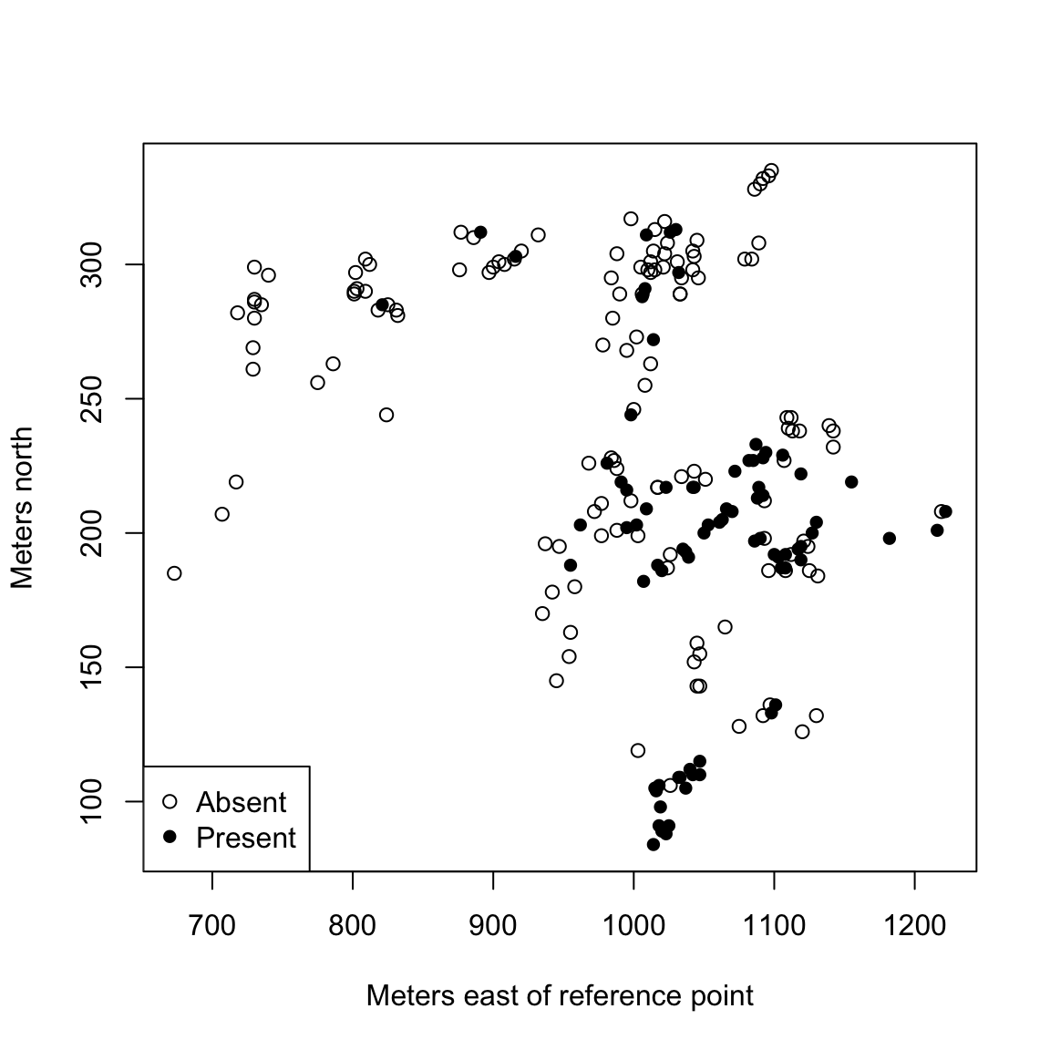
A natural goal is to under the relation between the occurence of a frog (pres.abs)
variable and the other geographic and environmental variables. This
naturally falls under the classification problem because the response
variable pres.abs is binary.
Email Spam Dataset
This dataset is from Chapter 10 of the book Data Analysis and Graphics using R. The original dataset is from the UC Irvine Repository of Machine Learning. The original dataset had 4607 observations and 57 explanatory variables. The authors of the book selected 6 of the 57 variables.
##   crl.tot dollar  bang money n000 make yesno
## 1     278  0.000 0.778  0.00 0.00 0.00     y
## 2    1028  0.180 0.372  0.43 0.43 0.21     y
## 3    2259  0.184 0.276  0.06 1.16 0.06     y
## 4     191  0.000 0.137  0.00 0.00 0.00     y
## 5     191  0.000 0.135  0.00 0.00 0.00     y
## 6 54 0.000 0.000 0.00 0.00 0.00 yThe main variable here is yesno which indicates if the email
is spam or not. The other variables are explanatory variables. They are:
crl.tot- total length of words that are in capitalsdollar- frequency of the $ symbol, as percentage of all charactersbang- freqency of the ! symbol, as a percentage of all characters,money- freqency of the word money, as a percentage of all words,n000- freqency of the text string 000, as percentage of all words,make- freqency of the word make, as a percentage of all words.
The goal is mainly to predict whether a future email is spam or not based on these explanatory variables. This is once again a classification problem because the response is binary.
There are, of course, many more examples where the classification problem arises naturally.
7.2 Logistic Regression Setup
We consider the simple example, where we just have a single predictor, \(x\). We could plot our \(y\) versus our \(x\), and might have something that looks like these two examples plotted below (this is toy data I made up):
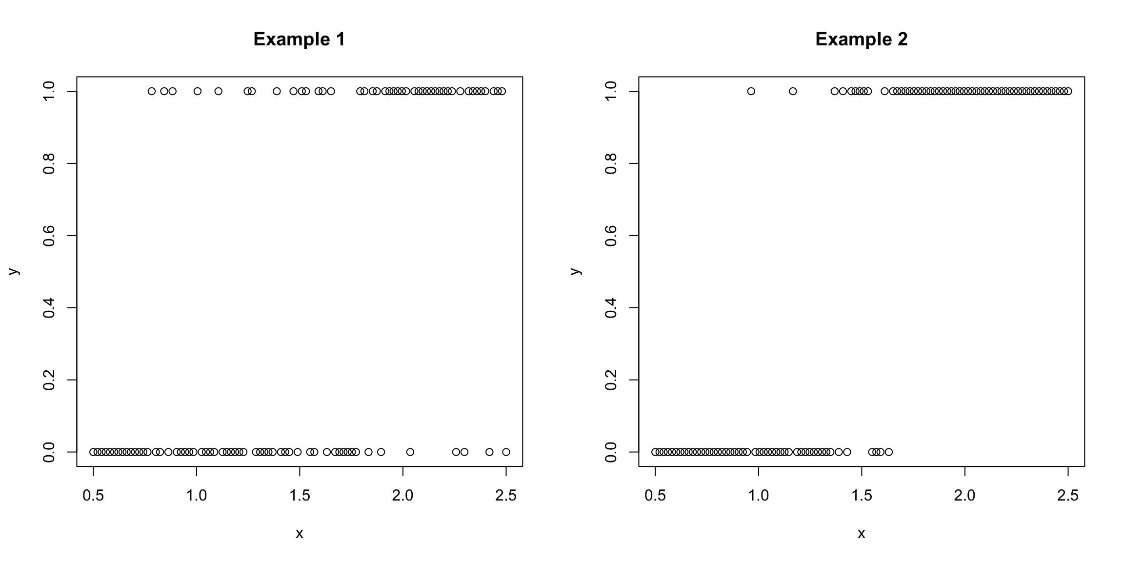
Our goal is to predict the value of \(y\) from our \(x\).
What do you notice about the relationship of \(y\) with \(x\) in the above two examples? In which of the two examples is it easier to predict \(y\)?
This is a standard x-y scatterplot from regression, but is a pretty lousy plot for binary data! How could you better illustrate this data?
Prediction of Probability
Logistic regression does not directly try to predict values 0 or 1, but instead tries to predict the probability that \(y\) is 1 as a function of its variables, \[p(x)=P(Y=1 | x)\] Note that this can be thought of as our model for the random process of how the data were generated: for a given value of \(x\), you calculate the \(p(x)\), and then toss a coin that has probability \(p(x)\) of heads. If you get a head, \(y=1\), otherwise \(y=0\).65 The coin toss provides the randomness – \(p(x)\) is an unknown but fixed quantity.
Note that unlike regression, we are not writing \(y\) as a function of \(x\) plus some noise (i.e. plus a random noise term). Instead we are writing \(P(Y=1)\) as a function of \(x\); our randomness comes from the random coin toss we perform once we know \(p(x)\).
We can use these probabilities to try to predict what the actual observed \(y\) is more likely to be (the classification problem). For example, if \(P(Y=1|x)>0.5\) we could decide to predict that \(y=1\) and otherwise \(y=0\); we could also use the probabilities to be more stringent. For example, we could predict \(y=1\) if \(P(Y=1|x)>0.7\) and \(y=0\) if \(P(Y=1|x)<0.3\) and otherwise not make a prediction. The point is that if we knew the probabilities, we could decide what level of error in either direction we were willing to make. We’ll discuss this more later in the chapter.
7.2.1 Estimating Probabilities
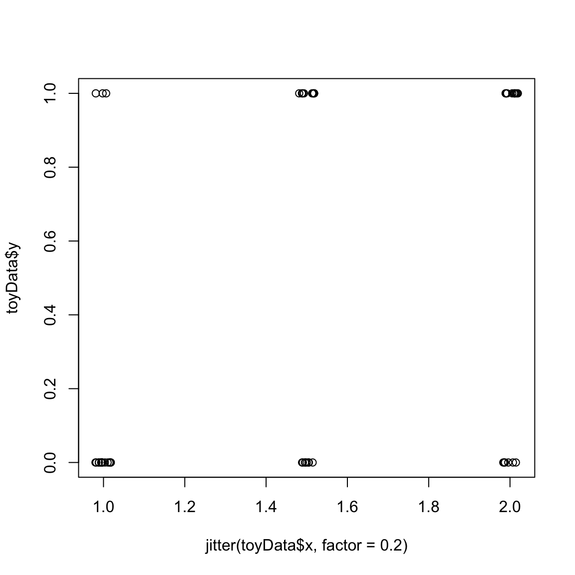
How can we estimate these probabilities? Let’s think of a simpler example, where we observe many observations but only at three values \(x\) (1, 1.5, and 2), and their corresponding \(y\). In the following plot I’ve added a small amount of noise to the \(x\) values so they don’t overplot on each other, but there are actually only three values:
We can see this is still not entirely sufficient to see precisely the proportion of 0 versus 1 values at each x value, so I will plot each x value as a separate barplot so we can directly compare the proportion of 0 versus 1 values at each x value:
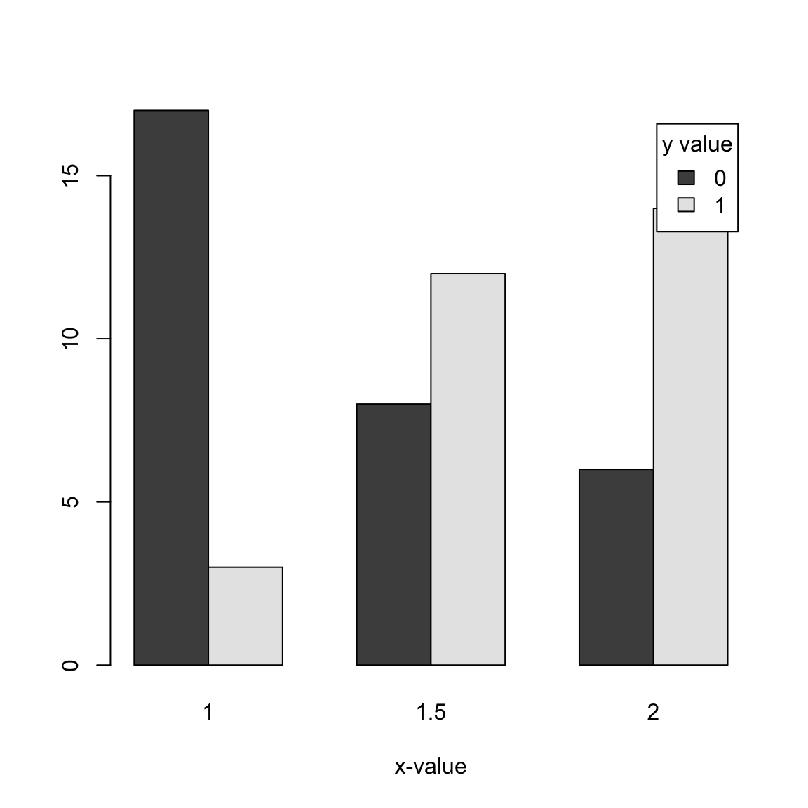
With this kind of data (i.e. with replication at each x-value), we could imagine estimating the probability that \(y=1\) if \(x=2\), for example: we could take the proportion of \(y=1\) values for the observations that have \(x=2\) (0.6. We could call this value \(\hat{p}(2)\). We could do this for each of the three values of \(x\), getting \(\hat{p}(1)\),\(\hat{p}(1.5)\),\(\hat{p}(2)\).
We could also then try to see how the probability of \(y=1\) is changing with \(x\). For example, if we plotted \(\hat{p}(x)\) from above we would have:
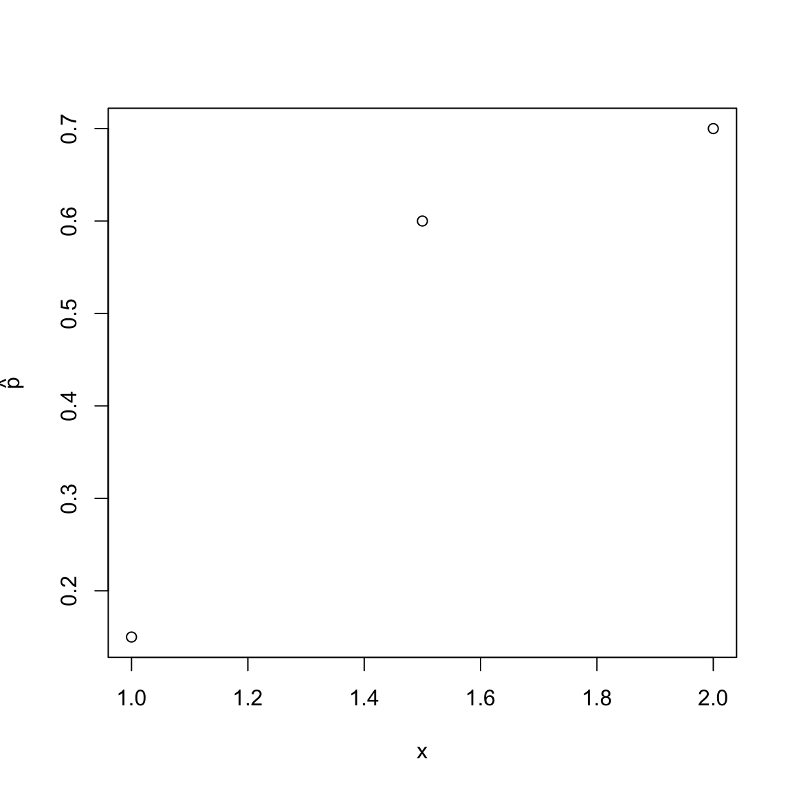
So in this example, we see an increase in the value \(\hat{p}(x)\) as \(x\) increases, i.e. the probability of \(y=1\) increases with \(x\). However, with only 3 values of \(x\) we couldn’t describe \(\hat{p}(x)\) as a function of \(x\) since we couldn’t say much about how \(\hat{p}(x)\) changes with \(x\) for other values.
But if we had this kind of data with a lot of different \(x\) values, we could think of a way to estimate how \(\hat{p}(x)\) is changing with \(x\), perhaps with curve fitting methods we’ve already considered.
Without repeated observations
More generally, however, we won’t have multiple observations with the same \(x\).
Returning to the more realistic toy data example I created earlier (“Example 1”), we only have one observation at each \(x\) value, but we have a lot of \(x\) values. Consider, for example, estimating the probability at \(x=2.5\) (colored in red). We only have one such value, and it’s \(y\) values is 0:
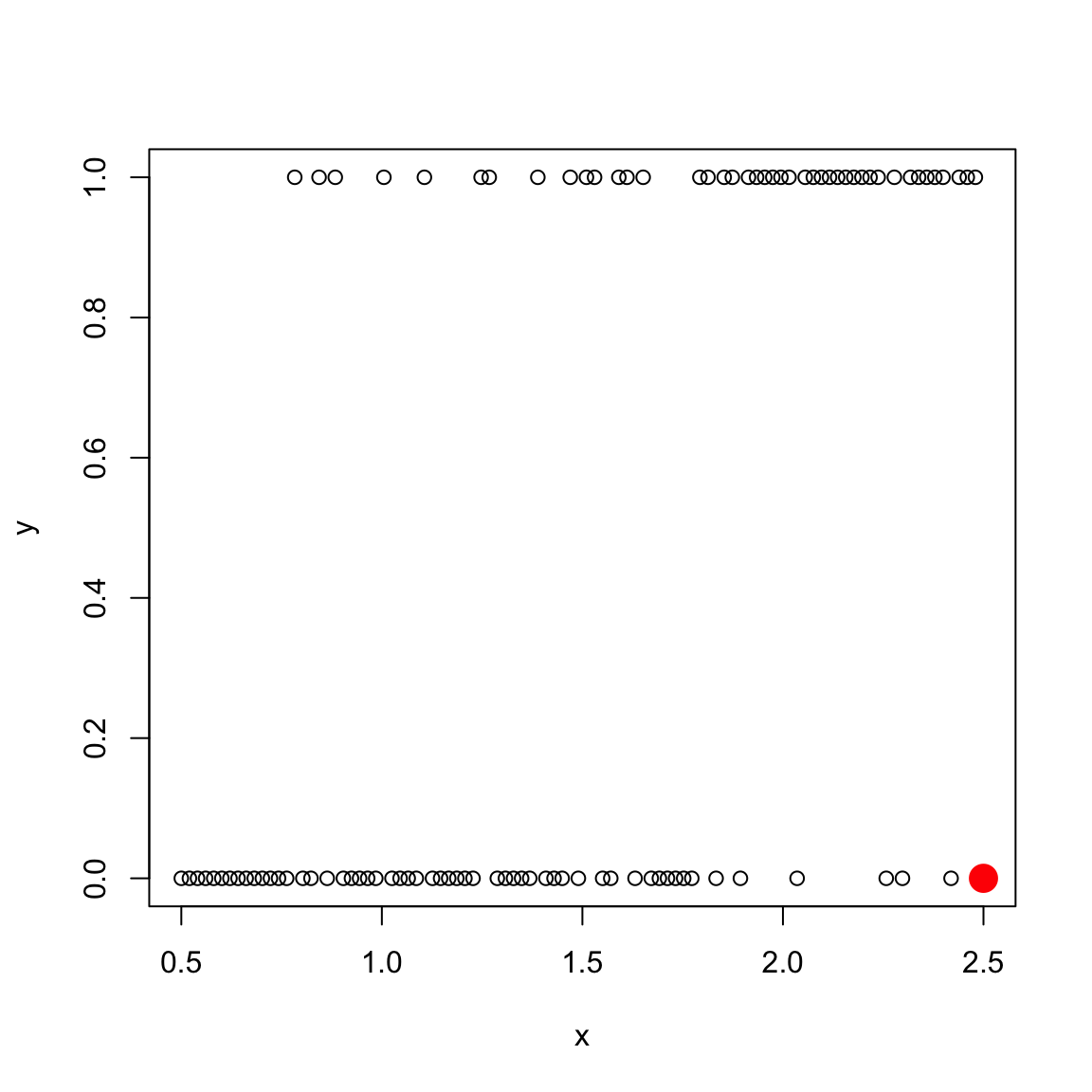
We only have 1 observation, and \(\hat{p}(2.5)=0\) is a very bad prediction based on 1 observation. Indeed, looking at the surrounding \(x\) values around it, it is clear from the plot that the probability that \(y=1\) when \(x=2.5\) is probably pretty high, though not \(1\). We happen to get \(y=0\) at \(x=2.5\), but that was probably random chance.
We could do something, like try to bin together similar \(x\) values and estimate a single probability for similar values of \(x\), like our local regression fitting in earlier chapters. Creating bins gets complicated when you have more than one explanatory variable (though we will see that we do something similar to this in decision trees, in the next chapter).
Instead, we will focus on predicting the function \(p(x)\) by assuming \(p(x)\) is a straightforward function of \(x\).
Why not regression?
We could ask, why don’t we just do regression to predict \(y\)? In other words, we could do standard regression with the observed \(y\) values as the response.
Numerically, we can do it, in the sense that lm will give us an answer that vaguely seems reasonable. Here is the result from fitting to the two example data sets from above (“Example 1” and “Example 2” from above):
par(mfrow = c(2, 2))
plot(y ~ x, data = toyDataCont, main = "Example 1")
abline(lm(y ~ x, data = toyDataCont))
plot(lm(y ~ x, data = toyDataCont), which = 1)
plot(y ~ x, data = toyDataCont2, main = "Example 2")
abline(lm(y ~ x, data = toyDataCont2))
plot(lm(y ~ x, data = toyDataCont2), which = 1)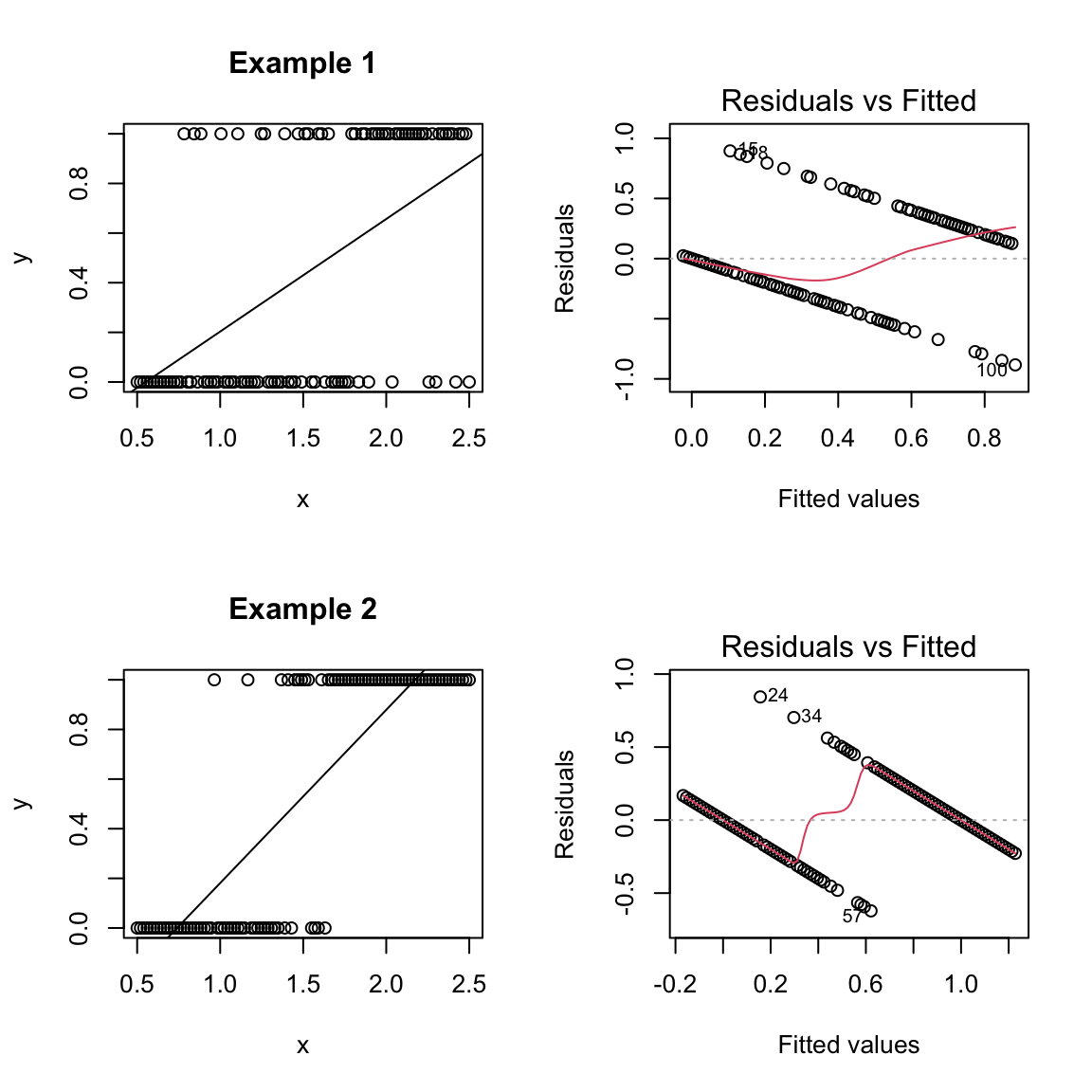
What do you notice about using these predicted lines as an estimate \(\hat{p}(x)\)?
This result doesn’t give us a prediction for probabilities (since values are outside of [0,1]).
What about forgetting about predicting the probability and just try to predict a 0 or 1 for y (i.e. classification)? The regression line doesn’t give us an obvious way to create a classification. We’d have to make some decision (based on our data) on what value of x to decide to make a prediction of 1 versus zero. Since we aren’t correctly predicting probabilities, there’s no obvious cutoff, though we could use our data to try to pick one.
7.2.2 Logit function / Log Odds
What do we do instead?
Instead, we want a function for \(p(x)\) that is constrained within [0,1]. While we could try to figure out such a function, we are instead going to take another tack which will lead us to such a function. Specifically, we are going to consider transforming our \(p(x)\) so that it takes on all real-valued values, say \[z(x)=\tau(p(x))\] Instead of trying to estimate \(p(x)\), we will try to estimate \(z(x)\) as a function of our \(x\).
Why? Because it will mean that \(z(x)\) is no longer constrained to be between 0 and 1. Therefore, we can be free to use any simple modeling we’ve already learned to estimate \(z(x)\) (for example linear regression) without worrying about any constraints. Then to get \(\hat{p}(x)\), we will invert to get \[\hat{p}(x)=\tau^{-1}(\hat{z}(x)).\] (Note that while \(p(x)\) and \(z(x)\) are unknown, we pick our function \(\tau\) so we don’t have to estimate it)
The other reason is that we are going to choose a function \(\tau\) such that the value \(z(x)\) is actually interpretable and makes sense on its own; thus the function \(z(x)\) is actually meaningful to estimate on its own.
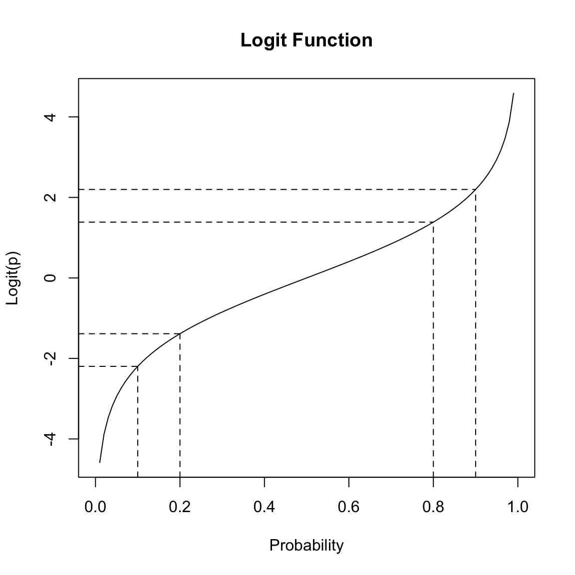
There are different reasonable choices for \(\tau\), but we are going to focus on the one traditionally used in logistic regression. The function we are going to use is called the logit function. It takes any value \(p\) in (0,1), and returns a real value: \[\tau(p)=logit(p)=log(\frac{p}{1-p}).\]
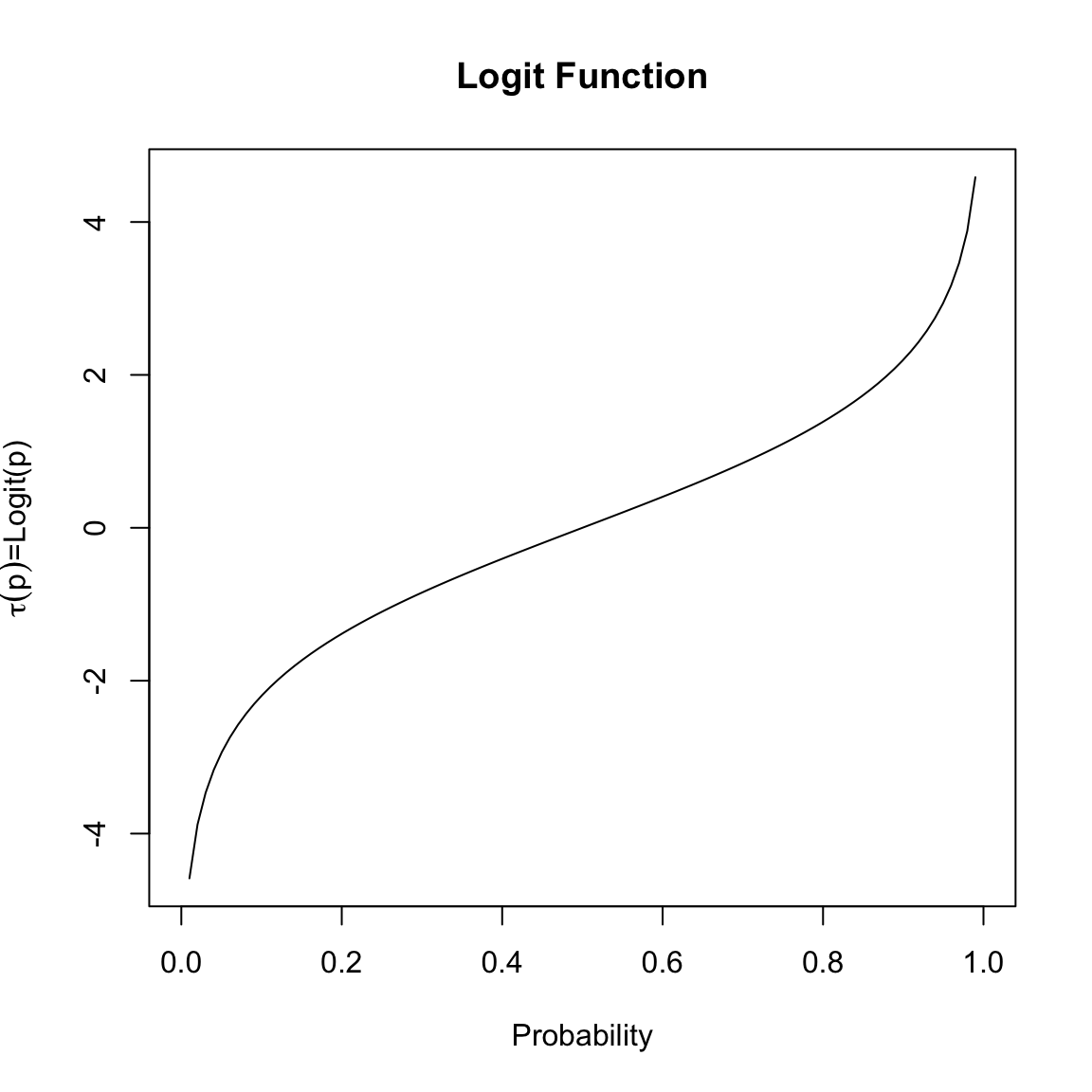
The value \(z=logit(p)\) is interpretable as the log of the odds, a common measure of discussing the probability of something.
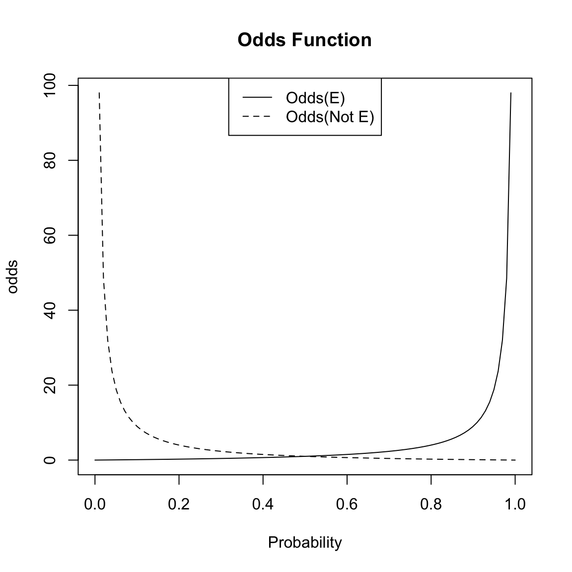
Odds
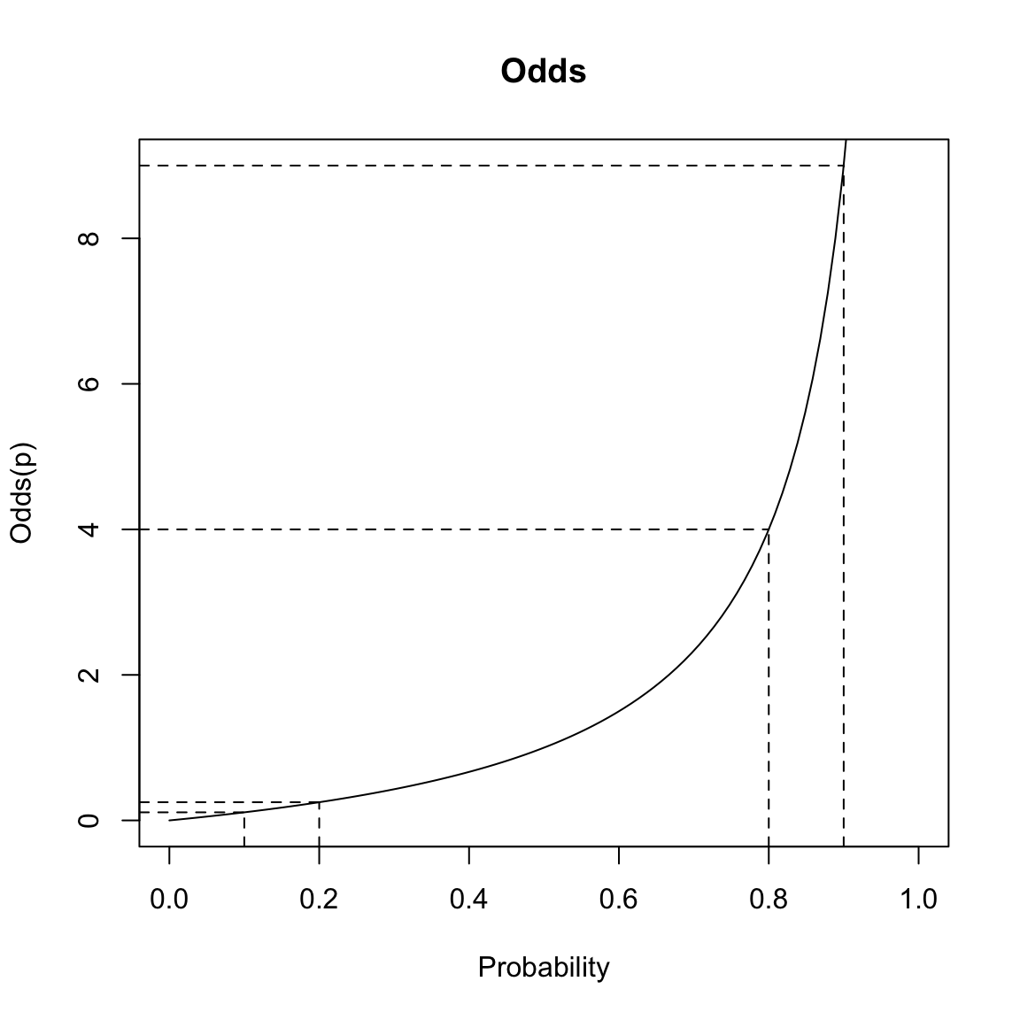
Let \(p\) be the probability of an event \(E\), \(p=P(E)\). For example, our event could be \(E=\{y =1\}\), and then \(p=P(E)=P (y =1 )\)). Then the odds of the event \(E\) is denoted by \(odds(E)\) and defined as \[\begin{equation*} odds(E) := \frac{P(E~ \text{happens})}{P(E ~\text{does not happen})} = \frac{P(E)}{1 - P(E)} = \frac{p}{1-p} \end{equation*}\] An important thing to note is that while \(p=P(E)\) lies between 0 and 1, the odds of \(E\) (\(odds(E)\)) is only restricted to be nonnegative – i.e. the odds takes on a wider range of values.
Note the following simple formulae relating probability and odds: \[\begin{equation*} p= P(E) = \frac{odds(E)}{1 + odds(E)} \end{equation*}\] So if you know the odds of an event, you can also calculate the probability of the event.
Log Odds
From a modeling perspective, it is still akward to work with odds – for example to try to predict the odds – because it must be positive. Moreover, it’s not symmetric in our choice of whether we consider \(P(y=1)\) versus \(P(y=0)\). Changing the probability of \(y=1\) from 0.8 to 0.9 create large differences in the odds, but similarly changing the probability from 0.2 to 0.1 create small changes in the odds.
 This is unfortunate, since the choice of trying to estimate \(P(y=1)\) is arbitrary – we could have just as easily considered \(P(y=0)\) and modeled that quantity.
However, if we take the log of the odds, there is no restriction on the value of \(\log (odds(E))\) i.e., \[log\left(\frac{p}{1-p}\right)\] As your probability \(p\) ranges between 0 and 1, the log-odds will take on all real-valued numbers. Moreover, the logit function is symmetric around 0.5, meaning that the difference between the log-odds of \(p=0.8\) versus \(p=0.9\) is the same difference as the log-odds of \(p=0.2\) versus \(p=0.1\):
Converting from log-odds to probability
As we discussed above, our goal is going to be to model \(z=logit(p)\), and then be able to transform from \(z\) back to \(p\).
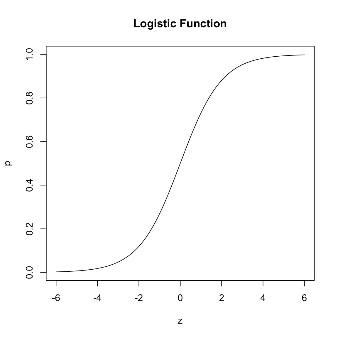
We have the simple relationship between \(z\) and the probability \(p\) \[\begin{equation*} p= P(E) = \tau^{-1}(z)= \frac{e^z}{1+e^z}=\frac{1}{1+e^{-z}}. \end{equation*}\] This function \(\tau^{-1}\) is called the logistic function. For any real-valued \(z\), the logistic function converts that number into a value between 0-1 (i.e. a probability).
7.2.3 Logistic Regression Model
Logistic regression, then, is to model the \(logit(p)\) (i.e. the log-odds of the event), as a linear function of the explanatory variable values \(x_i\) of the \(i^{th}\) individual. Again, this is a feasible thing to do, since \(\log odds\) take on the full range of values, so that we won’t have to figure out how to make sure we don’t predict probabilities outside of 0-1. Then, because of the relationships above, this gives us a model for the probabilities with respect to our explanatory variables \(x\).
The logistic regression model, for \(p=P(y = 1)\), is given as: \[\begin{equation*} \log(\frac{p}{1-p})=\log \left(odds(y = 1) \right) = \beta_0 + \beta_1 x_1 + \beta_2 x_2 + \dots + \beta_p x_p. \end{equation*}\]
This means that we are modeling the probabilities as \[\begin{equation*} p(x)=\frac{\exp(\beta_0 + \beta_1 x_1 + \beta_2 x_2 + \dots + \beta_p x_p)}{1+\exp(\beta_0 + \beta_1 x_1 + \beta_2 x_2 + \dots + \beta_p x_p)} \end{equation*}\]
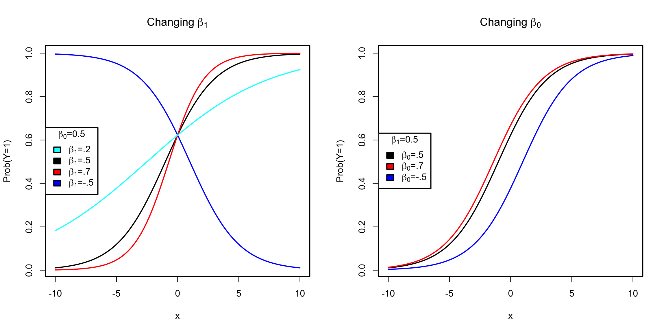
Visualizing Logistic Model
To understand the effect of these variables, let’s consider our model for a single variable x: \[log(\frac{p_i}{1-p_i})= \log(odds(y_i = 1)) = \beta_0+\beta_1 x_i\] which means \[p_i=\frac{\exp{(\beta_0+\beta_1 x_i)}}{1+exp(\beta_0+\beta_1 x_i)}\]
We can visualize the relationship of the probability \(p\) of getting \(y=1\) as a function of \(x\), for different values of \(\beta\)
Fitting the Logistic Model in R
The R function for logistic regression in R is
glm() and it is not very different from lm() in
terms of syntax.
For the frogs dataset, we will try to fit a model (but without the geographical variables)
frogsNoGeo <- frogs[, -c(2, 3)]
glmFrogs = glm(pres.abs ~ ., family = binomial, data = frogsNoGeo)
summary(glmFrogs)
##
## Call:
## glm(formula = pres.abs ~ ., family = binomial, data = frogsNoGeo)
##
## Deviance Residuals:
## Min 1Q Median 3Q Max
## -1.7215 -0.7590 -0.2237 0.8320 2.6789
##
## Coefficients:
## Estimate Std. Error z value Pr(>|z|)
## (Intercept) 1.105e+02 1.388e+02 0.796 0.42587
## altitude -3.086e-02 4.076e-02 -0.757 0.44901
## distance -4.800e-04 2.055e-04 -2.336 0.01949 *
## NoOfPools 2.986e-02 9.276e-03 3.219 0.00129 **
## NoOfSites 4.364e-02 1.061e-01 0.411 0.68077
## avrain -1.140e-02 5.995e-02 -0.190 0.84920
## meanmin 4.899e+00 1.564e+00 3.133 0.00173 **
## meanmax -5.660e+00 5.049e+00 -1.121 0.26224
## ---
## Signif. codes: 0 '***' 0.001 '**' 0.01 '*' 0.05 '.' 0.1 ' ' 1
##
## (Dispersion parameter for binomial family taken to be 1)
##
## Null deviance: 279.99 on 211 degrees of freedom
## Residual deviance: 198.74 on 204 degrees of freedom
## AIC: 214.74
##
## Number of Fisher Scoring iterations: 6GLM is not just the name of a function in R, but a general term that stands for Generalized Linear Model. Logistic regression
is a special case of a generalized linear model; the family = binomial clause in the function call above tells R to fit a logistic
regression equation to the data – namely what kind of function to use to determine whether the predicted probabilities fit our data.
7.3 Interpreting the Results
7.3.1 Coefficients
The parameter \(\beta_j\) is interpreted as the change in log-odds of the event \(y= 1\) for a unit change in the variable \(x_j\) provided all other explanatory variables are kept unchanged. Equivalently, \(e^{\beta_j}\) can be interpreted as the multiplicative change in odds due to a unit change in the variable \(x_j\) – provided all other explanatory variables are kept unchanged.
The R function provides estimates of the
parameters \(\beta_0, \dots, \beta_p\). For example, in the frogs
dataset, the estimated coefficient of the
variable NoOfPools is 0.02986. This is interpreted as the change in
log-odds of the event of finding a frog when the NoOfPools increases
by one (provided the other variables remain unchanged). Equivalently,
the odds of finding a frog get multiplied by \(\exp(0.02986) = 1.03031\)
when the NoOfPools increases by one.
P-values are also provided for each \(\hat{\beta}_j\); they have a similar interpretation as in linear regression, namely evaluating the null hypothesis that \(\beta_j=0\). We are not going to go into how these p-values are calculated. Basically, if the model is true, \(\hat{\beta}_j\) will be approximately normally distributed, with that approximation being better for larger sample size. Logistic regression significance statements rely much more heavily on asymptotics (i.e. having large sample sizes), even if the data exactly follows the data generation model!
7.3.2 Fitted Values and prediction
Now suppose a new site is found in the area for which the explanatory variable values are:
altitude=1700distance=400NoOfPools=30NoOfSites=8avrain=150meanmin=4meanmax=16
What can our logistic regression equation predict for the presence or absence of frogs in this area? Our logistic regression allows us to calculate the \(\log(odds)\) of finding frogs in this area as:
## [1] -13.58643Remember that this is \(\log(odds)\). From here, the odds of finding frogs is calculated as
## [1] 1.257443e-06These are very low odds. If one wants to obtain an estimate of the probability of finding frogs at this new location, we can use the formula above to get:
## [1] 1.257441e-06Therefore, we will predict that this species of frog will not be present at this new location.
Similar to fitted values in linear regression, we can obtain fitted
probabilities in logistic regression for each of the observations in
our sample using the fitted function:
## 2 3 4 5 6 7
## 0.9994421 0.9391188 0.8683363 0.7443973 0.9427198 0.7107780These fitted values are the fitted probabilities for each observation in our sample. For example, for \(i = 45\), we can also calculate the fitted value manually as:
i = 45
rrg = c(1, frogs$altitude[i], frogs$distance[i], frogs$NoOfPools[i],
frogs$NoOfSites[i], frogs$avrain[i], frogs$meanmin[i],
frogs$meanmax[i])
eta = sum(rrg * glmFrogs$coefficients)
prr = exp(eta)/(1 + exp(eta))
c(manual = prr, FittedFunction = unname(glmFrogs$fitted.values[i]))## manual FittedFunction
## 0.5807378 0.5807378The following plots the fitted values against the actual response:
boxplot(fitted(glmFrogs) ~ frogs$pres.abs, at = c(0,
1))
points(x = jitter(frogs$pres.abs), fitted(glmFrogs))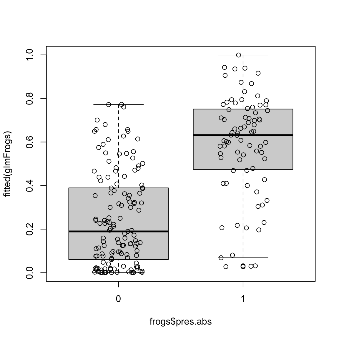
Why do I plot this as a boxplot?
Some of the regions where frogs were present seems to have received very low fitted probability under the model (and conversely, some of the regions with high fitted probability did not actually have any frogs). We can look at these unusual points in the following plot:
high0 <- frogs$pres.abs == 0 & glmFrogs$fitted > 0.7
low1 <- frogs$pres.abs == 1 & glmFrogs$fitted < 0.2
par(mfrow = c(1, 2))
plot(northing ~ easting, data = frogs, pch = c(1, 16)[frogs$pres.abs +
1], col = c("black", "red")[factor(high0)], xlab = "Meters east of reference point",
ylab = "Meters north", main = "Points with no frogs, but high prob")
plot(northing ~ easting, data = frogs, pch = c(1, 16)[frogs$pres.abs +
1], col = c("black", "red")[factor(low1)], xlab = "Meters east of reference point",
ylab = "Meters north", main = "Points with frogs, but low prob")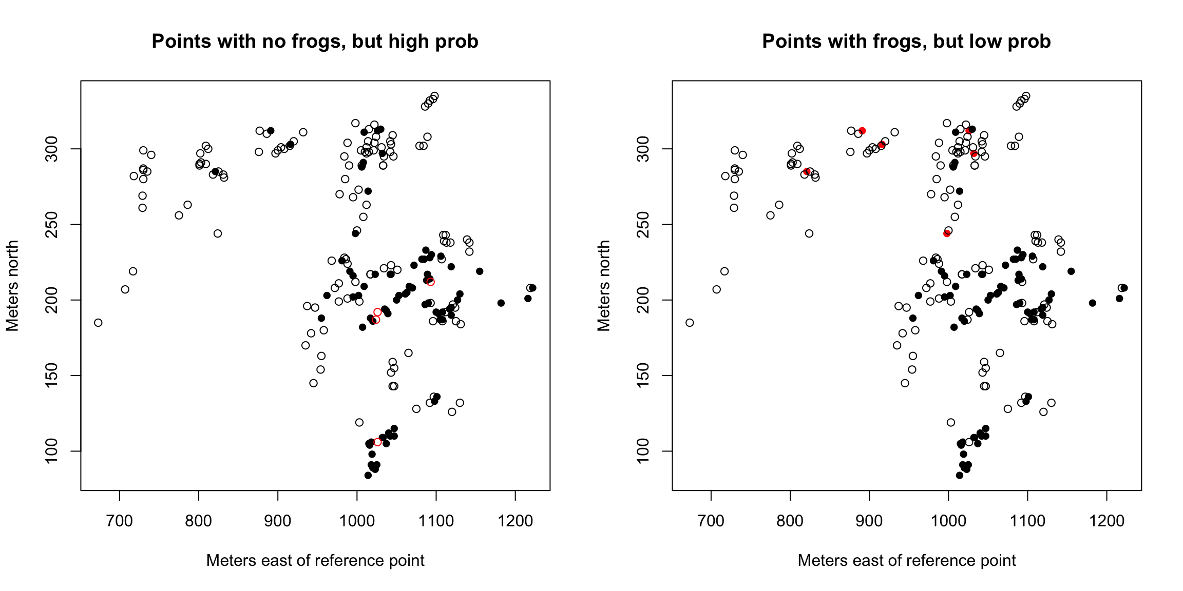
What do you notice about these points?
7.3.3 Fitting the model & Residual Deviance
We haven’t discussed how glm found the “best” choice of coefficients \(\beta\) for our model. Like regression, the coefficients are chosen based on getting the best fit to our data, but how we measure that fit is different for logistic regression.
In regression we considered the squared residual as a measure of our fit for each observation \(i\), \[(y_i-\hat{y}_i)^2,\] and minimizing the average fit to our data. We will do something similar in logistic regression, but
- We will consider the fit of the fitted probabilities
- The criterion we use to determine the best coefficients \(\beta\) is not the residual, but another notion of “fit” for every observation.
Let \(\hat{p}_1, \dots, \hat{p}_n\) denote the fitted probabilities in logistic regression for a possible vector of coefficients \(\beta_1,\ldots,\beta_p\). The actual response values are \(y_1, \dots, y_n\) (remember our responses \(y\) are binary, i.e. 0-1 values). If the fit is good, we would expect \(\hat{p}_i\) to be small (close to zero) when \(y_i\) is 0 and \(\hat{p}_i\) to be large (close to one) when \(y_i\) is 1. Conversely, if the fit is not good, we would expect \(\hat{p}_i\) to be large for some \(y_i\) that is zero and \(\hat{p}_i\) to be small for some \(y_i\) that is 1.
A commonly used function for measuring if a probability \(p\) is close to 0 is \[- 2 \log p.\] This quantity is always nonnegative and it becomes very large if \(p\) is close to zero. Similarly, one can measure if a probability \(p\) is close to 1 by \(- 2 \log (1 - p)\).
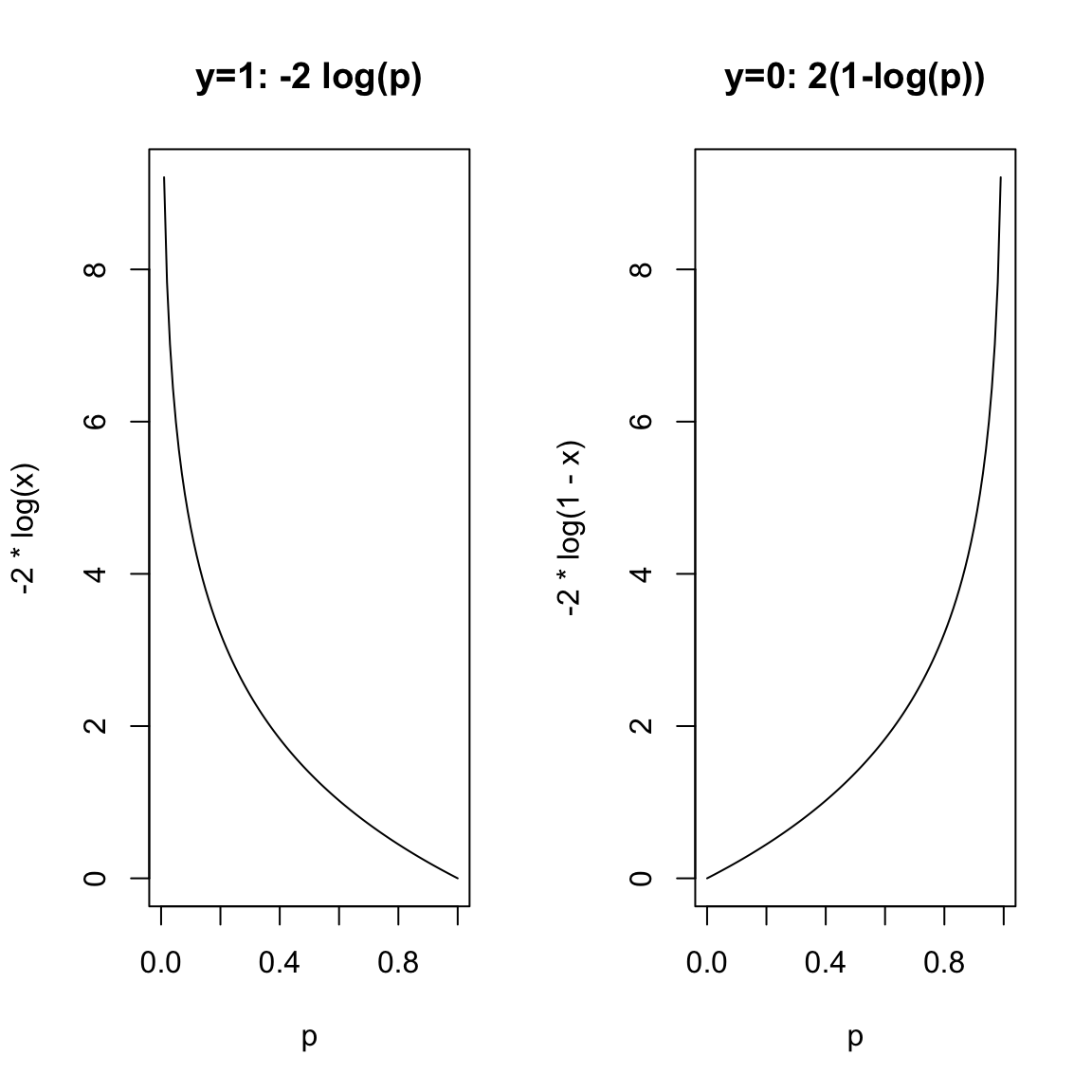
Using these quantities, we measure the quality of fit of \(\hat{p}_i\) to \(y_i\) by \[Dev(\hat{p}_i, y_i) = \left\{ \begin{array}{lr} -2\log \hat{p}_i & : y_i = 1\\ -2 \log \left(1 - \hat{p}_i \right) & : y_i = 0 \end{array} \right. \] This is called the deviance.66 If \(Dev(\hat{p}_i, y_i)\) is large, it means that \(\hat{p}_i\) is not a good fit for \(y_i\).
Because \(y_i\) is either 0 or 1, the
above formula for \(Dev(\hat{p}_i, y_i)\) can be written more succinctly
as
\[\begin{equation*}
Dev(\hat{p}_i, y_i) = y_i \left(- 2 \log \hat{p}_i \right) +
(1 - y_i) \left(- 2 \log (1 - \hat{p}_i) \right).
\end{equation*}\]
Note that this is the deviance for the \(i^{th}\) observation. We can get a measure
of the overall goodness of fit (across all observations) by simply
summing this quantity over all our observations. The resulting quantity
is called the Residual Deviance:
\[\begin{equation*}
RD = \sum_{i=1}^n Dev(\hat{p}_i, y_i).
\end{equation*}\]
Just like RSS, small values of \(RD\) are preferred and large values
indicate lack of fit.
This doesn’t have our \(\beta_j\) anywhere, so how does this help in choosing the best \(\beta\)? Well, remember that our fitted values \(\hat{p}_i\) is a specific function of our \(x_i\) values: \[\hat{p}_i=\hat{p}(x_i)=\tau^{-1}(\hat{\beta}_0+\ldots+\hat{\beta}_p x_i^{(p)})=\frac{\exp(\hat{\beta}_0+\ldots+\hat{\beta}_px_i^{(p)})}{1+\exp(\hat{\beta}_0+\ldots+\hat{\beta}_px_i^{(p)})}\] So we can put those values into our equation above, and find the \(\hat{\beta}_j\) that maximize that quantity. Unlike linear regression, this has to be maximized by a computer – you can’t write down a mathematical expression for the \(\hat{\beta}_j\) that minimize the residual deviance.
Residual Deviance in R
The function deviance can be used in R to calculate
deviance. It can, of course, also be calculated manually using the
fitted probabilities.
RD (Residual Deviance) can be calculated from our glm object as
## [1] 198.73847.4 Comparing Models
7.4.1 Deviance and submodels
Residual Deviance has parallels to RSS in linear regression, and we can use deviance to compare models similarly to linear regression.
RD decreases as you add variables
Just like the RSS in linear regression, the RD in logistic regression
will always decrease as more variables are added to the model. For example, in the
frogs dataset, if we remove the variable NoOfPools, the RD
changes to:
m2 = glm(pres.abs ~ altitude + distance + NoOfSites +
avrain + meanmin + meanmax, family = binomial,
data = frogs)
deviance(m2)## [1] 210.8392## [1] 198.7384Note that RD decreased from 210.84 to 198.7384 by adding NoOfPools.
The Null Model (No Variables)
We can similarly ask whether we need any of the variables (like the F test). The Null Deviance (ND) is the analogue of TSS (Total Sum of Squares) in linear regression. It simply refers to the deviance when there are no explanatory variables i.e., when one does logistic regression with only the intercept.
We can fit a model in R with no variables with the following syntax:
## [1] 279.987Note, when there are no explanatory variables, the fitted probabilities are all equal to \(\bar{y}\):
## 2 3 4 5 6 7
## 0.3726415 0.3726415 0.3726415 0.3726415 0.3726415 0.3726415## [1] 0.3726415Notice that this null deviance is reported in the summary of the full model we fit:
##
## Call:
## glm(formula = pres.abs ~ ., family = binomial, data = frogsNoGeo)
##
## Deviance Residuals:
##     Min       1Q   Median       3Q      Max
## -1.7215  -0.7590  -0.2237   0.8320   2.6789
##
## Coefficients:
##               Estimate Std. Error z value Pr(>|z|)
## (Intercept)  1.105e+02  1.388e+02   0.796  0.42587
## altitude    -3.086e-02  4.076e-02  -0.757  0.44901
## distance    -4.800e-04  2.055e-04  -2.336  0.01949 *
## NoOfPools    2.986e-02  9.276e-03   3.219  0.00129 **
## NoOfSites    4.364e-02  1.061e-01   0.411  0.68077
## avrain      -1.140e-02  5.995e-02  -0.190  0.84920
## meanmin      4.899e+00  1.564e+00   3.133  0.00173 **
## meanmax     -5.660e+00  5.049e+00  -1.121  0.26224
## ---
## Signif. codes:  0 '***' 0.001 '**' 0.01 '*' 0.05 '.' 0.1 ' ' 1
##
## (Dispersion parameter for binomial family taken to be 1)
##
##     Null deviance: 279.99  on 211  degrees of freedom
## Residual deviance: 198.74  on 204  degrees of freedom
## AIC: 214.74
##
## Number of Fisher Scoring iterations: 6Significance of submodels
The deviances come with degrees of freedom. The degrees of freedom of RD is \(n - p - 1\) (exactly equal to the residual degrees of freedom in linear regression) while the degrees of freedom of ND is \(n-1\).
Unlike regression, the automatic summary does not give a p-value as to whether this is a significant change in deviance. Similarly, the anova function for comparing submodels doesn’t give a significance for comparing a submodel to the larger model
## Analysis of Deviance Table
##
## Model 1: pres.abs ~ 1
## Model 2: pres.abs ~ altitude + distance + NoOfPools + NoOfSites + avrain +
##     meanmin + meanmax
##   Resid. Df Resid. Dev Df Deviance
## 1       211     279.99
## 2       204     198.74  7   81.249
The reason for this that because for logistic regression, unlike linear regression, there are multiple tests that for the same test. Furthermore, the glm function can fit other models than just the logistic model, and depending on those models, you will want different tests. I can specify a test, and get back a significance value:
## Analysis of Deviance Table
##
## Model 1: pres.abs ~ 1
## Model 2: pres.abs ~ altitude + distance + NoOfPools + NoOfSites + avrain +
##     meanmin + meanmax
##   Resid. Df Resid. Dev Df Deviance  Pr(>Chi)
## 1       211     279.99
## 2       204     198.74  7   81.249 7.662e-15 ***
## ---
## Signif. codes:  0 '***' 0.001 '**' 0.01 '*' 0.05 '.' 0.1 ' ' 1
What are the conclusions of these tests?
Comparison with Tests of \(\hat{\beta}_j\)
Notice that unlike linear regression, you get slightly different answers testing the importance of leaving out NoOfPools using the anova above and test statistics that come with the summary of the logistic object:
## Analysis of Deviance Table
##
## Model 1: pres.abs ~ altitude + distance + NoOfSites + avrain + meanmin +
##     meanmax
## Model 2: pres.abs ~ altitude + distance + NoOfPools + NoOfSites + avrain +
##     meanmin + meanmax
##   Resid. Df Resid. Dev Df Deviance Pr(>Chi)
## 1       205     210.84
## 2       204     198.74  1   12.101 0.000504 ***
## ---
## Signif. codes: 0 '***' 0.001 '**' 0.01 '*' 0.05 '.' 0.1 ' ' 1## Summary results:## Estimate Std. Error z value Pr(>|z|)
## (Intercept) 110.4935 138.7622 0.7963 0.4259
## altitude -0.0309 0.0408 -0.7571 0.4490
## distance -0.0005 0.0002 -2.3360 0.0195
## NoOfPools 0.0299 0.0093 3.2192 0.0013
## NoOfSites 0.0436 0.1061 0.4114 0.6808
## avrain -0.0114 0.0599 -0.1901 0.8492
## meanmin 4.8991 1.5637 3.1329 0.0017
## meanmax -5.6603 5.0488 -1.1211 0.2622They are still testing the same null hypothesis, but they are making different choices about the statistic to use67; in linear regression the different choices converge to the same test (the \(F\)-statistic for ANOVA is the square of the \(t\)-statistic), but this is a special property of normal distribution. Theoretically these two choices are equivalent for large enough sample size; in practice they can differ.
7.4.2 Variable Selection using AIC
Although the Residual Deviance (RD) measures goodness of fit, it cannot be used for variable selection because the full model will have the smallest RD. The AIC however can be used as a goodness of fit criterion (this involves selecting the model with the smallest AIC).
AIC
We can similarly calculate the AIC , only now it is based on the residual deviance, \[\begin{equation*} AIC = RD + 2 \left(p + 1 \right) \end{equation*}\]
## [1] 214.7384Based on AIC, we have the same choices as in linear regression.
In principle, one can go over all possible submodels and select the
model with the smallest value of AIC. But this involves going over
\(2^p\) models which might be computationally difficult if \(p\) is
moderate or large. A useful alternative is to use stepwise methods, only now comparing the change in RD rather than RSS; we can use the same step
function in R:
##
## Call:  glm(formula = pres.abs ~ distance + NoOfPools + meanmin + meanmax,
##     family = binomial, data = frogsNoGeo)
##
## Coefficients:
## (Intercept)     distance    NoOfPools      meanmin      meanmax
##  14.0074032   -0.0005138    0.0285643    5.6230647   -2.3717579
##
## Degrees of Freedom: 211 Total (i.e. Null);  207 Residual
## Null Deviance:       280
## Residual Deviance: 199.6     AIC: 209.6
7.5 Classification Using Logistic Regression
Suppose that, for a new site, our logistic regression model predicts that the probability that a frog will be found at that site to be \(\hat{p}(x)\). What if we want to make a binary prediction, rather than just a probability, i.e. prediction \(\hat{y}\) that is a 1 or 0, prediction whether there will be frogs found at that site. How large should \(\hat{p}(x)\) be so that we predict that frogs will be found at that site? 0.5 sounds like a fair threshold but would 0.6 be better?
Let us now introduce the idea of a confusion matrix. Given any chosen threshold, we can form obtain predictions in terms of 0 and 1 for each of the sample observations by applying the threshold to the fitted probabilities given by logistic regression. The confusion matrix is created by comparing these predictions with the actual observed responses.
| \(\hat{y} = 0\) | \(\hat{y} = 1\) | |
| \(y = 0\) | \(C_0\) | \(W_{1}\) |
| \(y = 1\) | \(W_0\) | \(C_{1}\) |
- \(C_0\) denotes the number of observations where we were correct in predicting 0: both the observed response as well as our prediction are equal to zero.
- \(W_{1}\) denotes the number of observations where were wrong in our predictions of 1: the observed response equals 0 but our prediction equals 1.
- \(W_{0}\) denotes the number of observations where were wrong in our predictions of 0: the observed response equals 1 but our prediction equals 0.
- \(C_1\) denotes the number of observations where we were correct in predicting 0: both the observed response as well as our prediction are equal to 1.
For example, for the frogs data, if we choose the threshold \(0.5\), then the entries of the confusion matrix can be calculated as:
## Confusion matrix for threshold 0.5:| \(\hat{y} = 0\) | \(\hat{y} = 1\) | |
| \(y = 0\) | \(C_0=112\) | \(W_1=21\) |
| \(y = 1\) | \(W_0=21\) | \(C_1=58\) |
On the other hand, if we use a threshold of \(0.3\), the numbers will be:
## Confusion for threshold 0.3:| \(\hat{y} = 0\) | \(\hat{y} = 1\) | |
| \(y = 0\) | \(C_0=84\) | \(W_1=49\) |
| \(y = 1\) | \(W_0=10\) | \(C_1=69\) |
Note that \(C_0\) and \(C_1\) denote the extent to which the response agrees with our threshold. And \(W_1\) and \(W_0\) measure the extent to which they disagree. An optimal threshold can be chosen to be one which minimizes \(W_1+W_0\). We can compute the entries of the confusion matrix for a range of possible thresholds.
##       C0  W1 W0 C1
## 0      0 133  0 79
## 0.05  33 100  3 76
## 0.1   47  86  5 74
## 0.15  61  72  5 74
## 0.2   69  64  6 73
## 0.25  80  53 10 69
## 0.3   84  49 10 69
## 0.35  91  42 13 66
## 0.4  100  33 14 65
## 0.45 106  27 18 61
## 0.5  112  21 21 58
## 0.55 118  15 26 53
## 0.6  121  12 35 44
## 0.65 126   7 44 35
## 0.7  129   4 50 29
## 0.75 130   3 59 20
## 0.8  133   0 69 10
## 0.85 133   0 71  8
## 0.9  133   0 73  6
## 0.95 133   0 78  1
## 1    133   0 79  0
Notice that I can get either \(W_1\) or \(W_0\) exactly equal to 0 (i.e no mis-classifications).
Why is it not a good idea to try to get \(W_1\) exactly equal to 0 (or alternatively try to get \(W_0\) exactly equal to 0)?
We can then plot the value of \(W_1+W_0\) for each value of the threshold in the following plot:
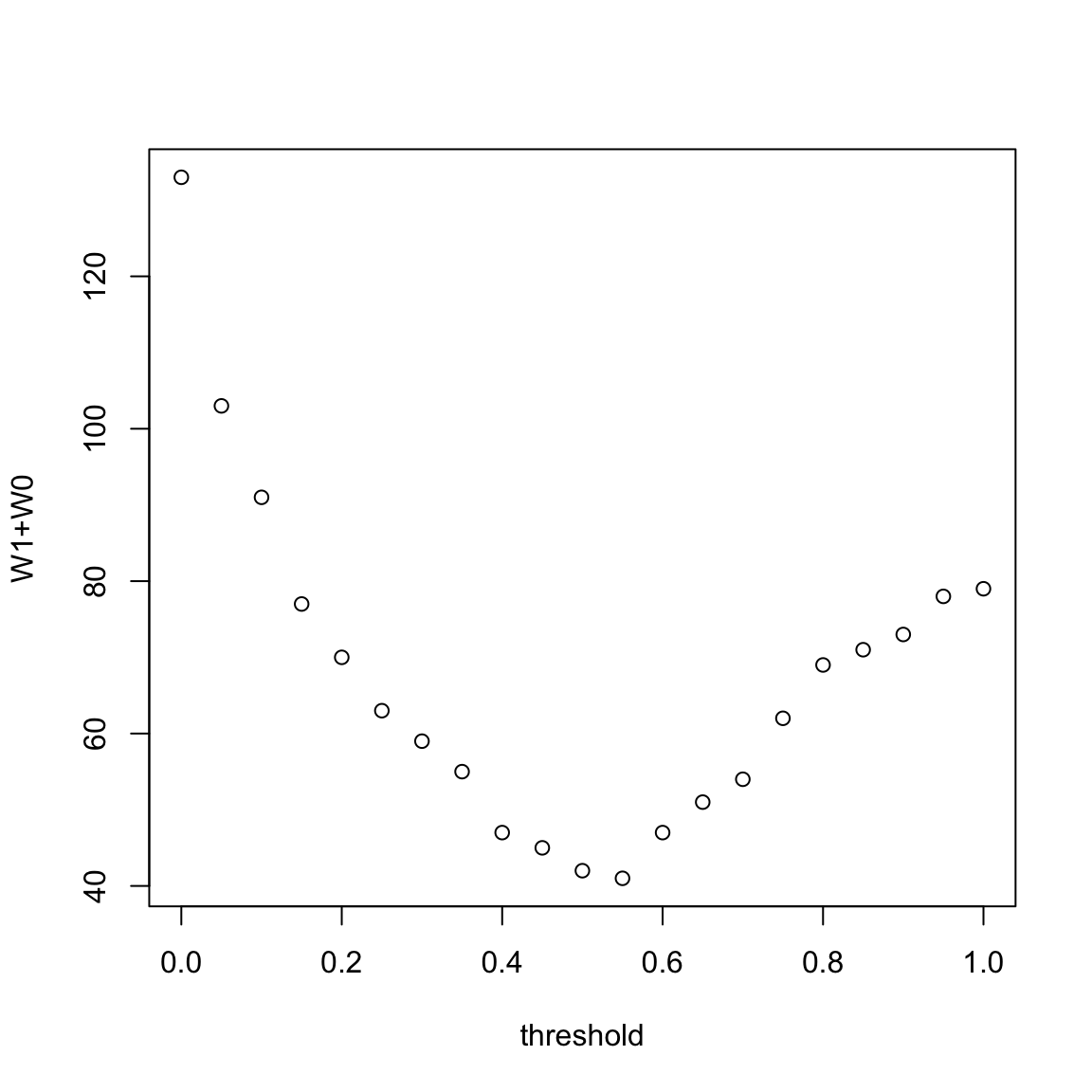
The smallest value of \(W_1+W_0\) corresponds to the threshold \(0.55\). It is sensible therefore to use this threshold for predictions.
But there might be settings where you want to allow more of one type of mistake than another. For example, you might prefer to detect a higher percentage of persons with a communicable disease, so as to limit the chances that someone further transmits the disease, even if that means slightly more people are wrongly told that they have the disease. These are trade-offs that frequently have to be made based on domain knowledge.
7.5.1 Example of Spam Dataset
Let us now consider the email spam dataset. Recall the dataset:
##   crl.tot dollar  bang money n000 make yesno
## 1     278  0.000 0.778  0.00 0.00 0.00     y
## 2    1028  0.180 0.372  0.43 0.43 0.21     y
## 3    2259  0.184 0.276  0.06 1.16 0.06     y
## 4     191  0.000 0.137  0.00 0.00 0.00     y
## 5     191  0.000 0.135  0.00 0.00 0.00     y
## 6      54  0.000 0.000  0.00 0.00 0.00     y
Before fitting a logistic regression model, let us first look at the summary and histograms of the explanatory variables:
##     crl.tot            dollar             bang             money
##  Min.   :    1.0   Min.   :0.00000   Min.   : 0.0000   Min.   : 0.00000
##  1st Qu.:   35.0   1st Qu.:0.00000   1st Qu.: 0.0000   1st Qu.: 0.00000
##  Median :   95.0   Median :0.00000   Median : 0.0000   Median : 0.00000
##  Mean   :  283.3   Mean   :0.07581   Mean   : 0.2691   Mean   : 0.09427
##  3rd Qu.:  266.0   3rd Qu.:0.05200   3rd Qu.: 0.3150   3rd Qu.: 0.00000
##  Max.   :15841.0   Max.   :6.00300   Max.   :32.4780   Max.   :12.50000
##       n000             make        yesno
##  Min.   :0.0000   Min.   :0.0000   n:2788
##  1st Qu.:0.0000   1st Qu.:0.0000   y:1813
##  Median :0.0000   Median :0.0000
##  Mean   :0.1016   Mean   :0.1046
##  3rd Qu.:0.0000   3rd Qu.:0.0000
## Max. :5.4500 Max. :4.5400par(mfrow = c(3, 2))
for (i in 1:5) hist(spam[, i], main = "", xlab = names(spam)[i],
breaks = 10000)
par(mfrow = c(1, 1))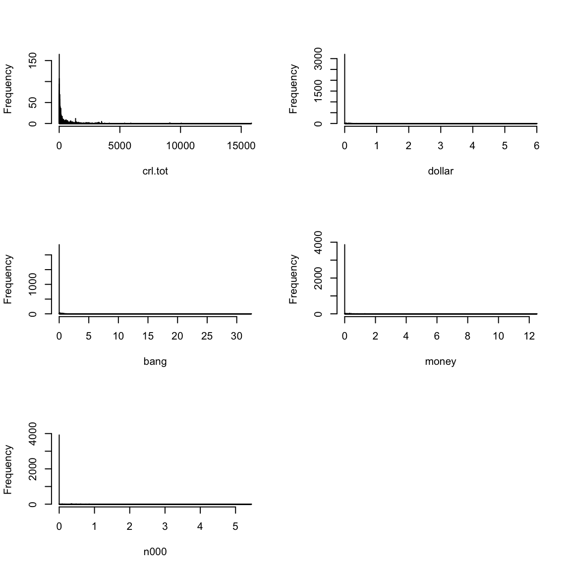
The following is a pairs plot of the variables.
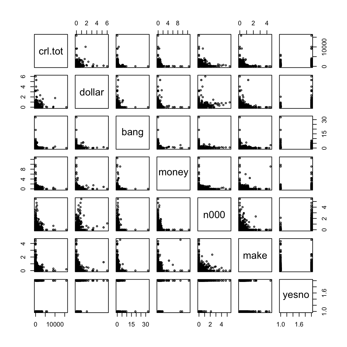
It is clear from these plots that the explanatory variables are highly skewed and it is hard to see any structure in these plots. Visualization will be much easier if we take logarithms of the explanatory variables.
s = 0.001
pairs(~log(crl.tot) + log(dollar + s) + log(bang +
    s) + log(money + s) + log(n000 + s) + log(make +
    s) + yesno, data = spam, cex = 0.5)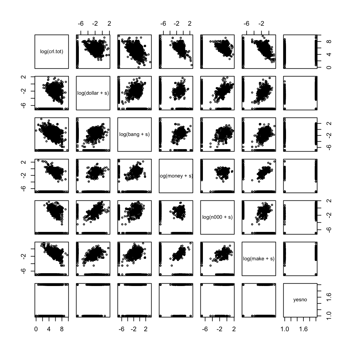
We now fit a logistic regression model for \(yesno\) based on the logged explanatory variables.
spam.glm <- glm(yesno ~ log(crl.tot) + log(dollar +
    s) + log(bang + s) + log(money + s) + log(n000 +
    s) + log(make + s), family = binomial, data = spam)
summary(spam.glm)
##
## Call:
## glm(formula = yesno ~ log(crl.tot) + log(dollar + s) + log(bang +
## s) + log(money + s) + log(n000 + s) + log(make + s), family = binomial,
## data = spam)
##
## Deviance Residuals:
## Min 1Q Median 3Q Max
## -3.1657 -0.4367 -0.2863 0.3609 2.7152
##
## Coefficients:
## Estimate Std. Error z value Pr(>|z|)
## (Intercept) 4.11947 0.36342 11.335 < 2e-16 ***
## log(crl.tot) 0.30228 0.03693 8.185 2.71e-16 ***
## log(dollar + s) 0.32586 0.02365 13.777 < 2e-16 ***
## log(bang + s) 0.40984 0.01597 25.661 < 2e-16 ***
## log(money + s) 0.34563 0.02800 12.345 < 2e-16 ***
## log(n000 + s) 0.18947 0.02931 6.463 1.02e-10 ***
## log(make + s) -0.11418 0.02206 -5.177 2.25e-07 ***
## ---
## Signif. codes: 0 '***' 0.001 '**' 0.01 '*' 0.05 '.' 0.1 ' ' 1
##
## (Dispersion parameter for binomial family taken to be 1)
##
## Null deviance: 6170.2 on 4600 degrees of freedom
## Residual deviance: 3245.1 on 4594 degrees of freedom
## AIC: 3259.1
##
## Number of Fisher Scoring iterations: 6Note that all the variables are significant. We actually could have fitted a linear model as well (even though the response variable is binary).
spam.lm <- lm(as.numeric(yesno == "y") ~ log(crl.tot) +
    log(dollar + s) + log(bang + s) + log(money + s) +
    log(n000 + s) + log(make + s), data = spam)
summary(spam.lm)
##
## Call:
## lm(formula = as.numeric(yesno == "y") ~ log(crl.tot) + log(dollar +
## s) + log(bang + s) + log(money + s) + log(n000 + s) + log(make +
## s), data = spam)
##
## Residuals:
## Min 1Q Median 3Q Max
## -1.10937 -0.13830 -0.05674 0.15262 1.05619
##
## Coefficients:
## Estimate Std. Error t value Pr(>|t|)
## (Intercept) 1.078531 0.034188 31.547 < 2e-16 ***
## log(crl.tot) 0.028611 0.003978 7.193 7.38e-13 ***
## log(dollar + s) 0.054878 0.002934 18.703 < 2e-16 ***
## log(bang + s) 0.064522 0.001919 33.619 < 2e-16 ***
## log(money + s) 0.039776 0.002751 14.457 < 2e-16 ***
## log(n000 + s) 0.018530 0.002815 6.582 5.16e-11 ***
## log(make + s) -0.017380 0.002370 -7.335 2.61e-13 ***
## ---
## Signif. codes: 0 '***' 0.001 '**' 0.01 '*' 0.05 '.' 0.1 ' ' 1
##
## Residual standard error: 0.3391 on 4594 degrees of freedom
## Multiple R-squared: 0.5193, Adjusted R-squared: 0.5186
## F-statistic: 827.1 on 6 and 4594 DF, p-value: < 2.2e-16A comparison plot of the fitted values for the linear regression and logistic regression is given below.
par(mfrow = c(1, 1))
plot(spam.lm$fitted.values, spam.glm$fitted.values,
    asp = 1)
abline(c(0, 1), col = "red")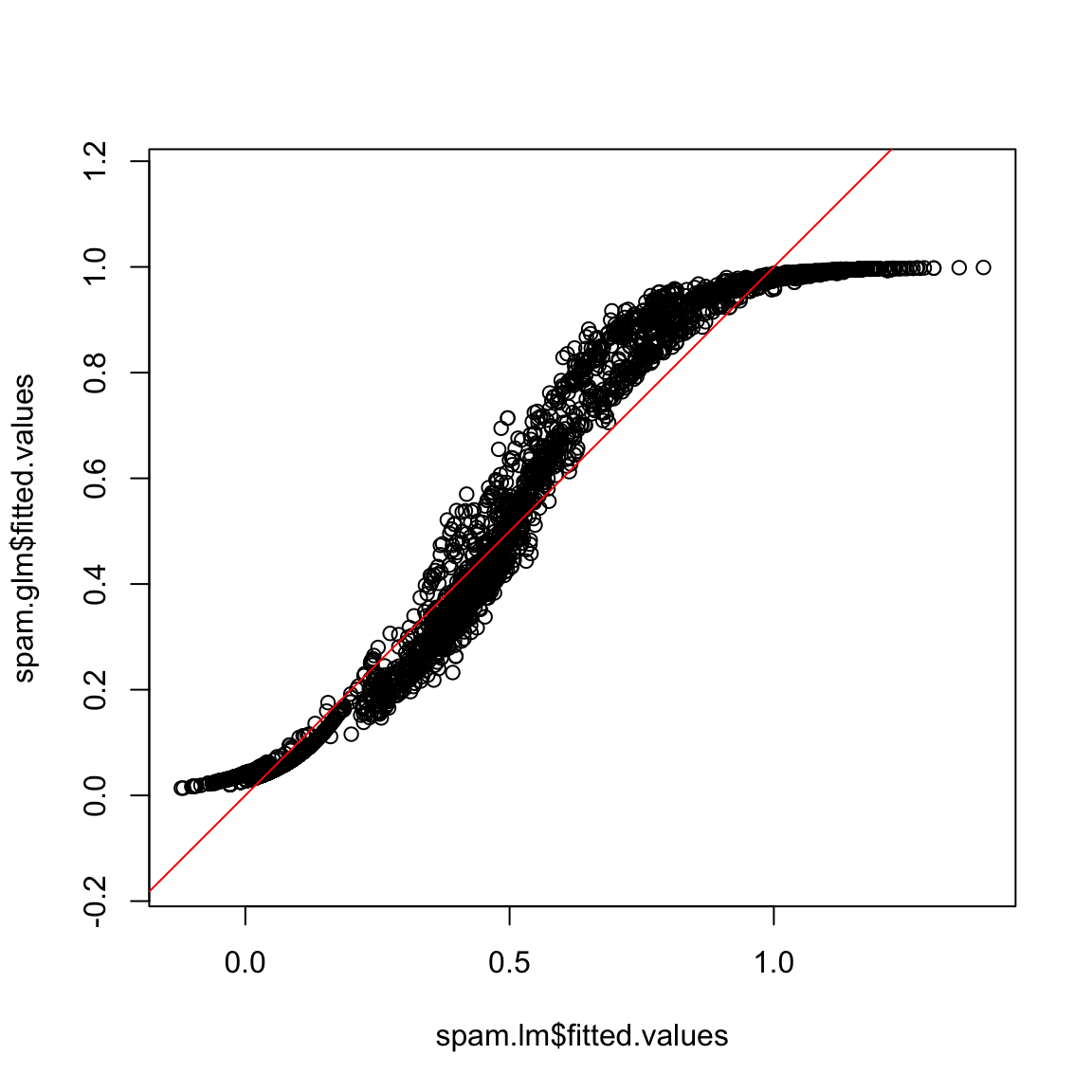
Note that some of the fitted values for the linear model are less than 0 and some are more than one. We can formally compare the prediction performance of the linear model and the generalized linear model by the confusion matrix. For various thresholds on the fitted values, the confusion matrices of linear regression and logistic regression can be computed and we can compare their misclassification error
v <- seq(0.001, 0.999, length = 50)
y <- as.numeric(spam$yesno == "y")
glm.conf <- confusion(y, spam.glm$fitted, v)
lm.conf <- confusion(y, spam.lm$fitted, v)
matplot(v, cbind((glm.conf[, "W1"] + glm.conf[, "W0"])/4601,
    (lm.conf[, "W1"] + lm.conf[, "W0"])/4601), xlab = "threshold",
    ylab = "W0+W1", type = "b", pch = 1)
legend(0.8, 0.4, lty = 1:2, col = 1:2, c("glm", "lm"))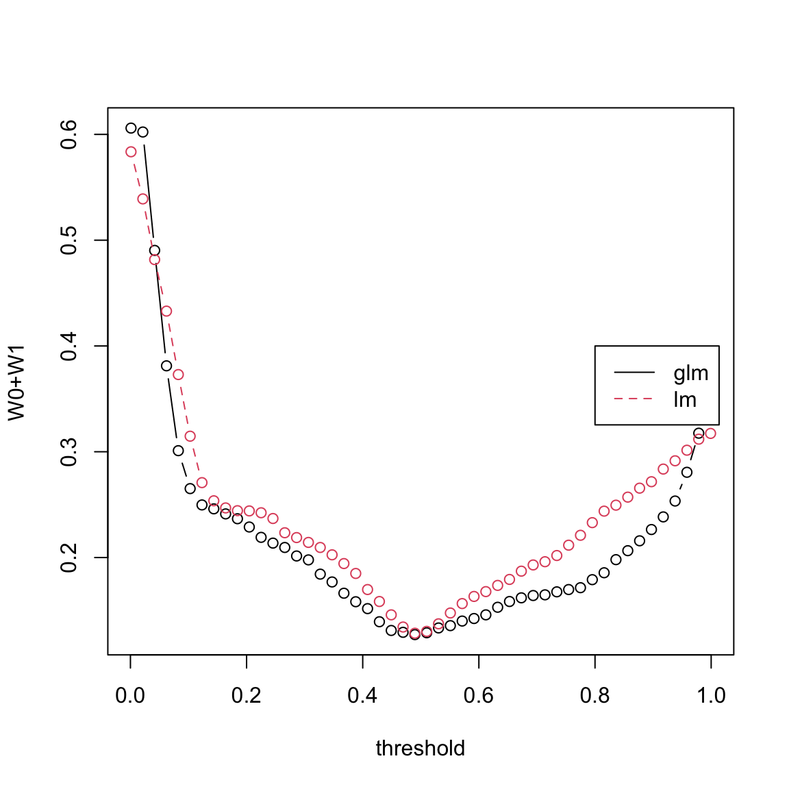
It is clear from this plot that 0.5 is the best threshold for both linear and logistic regression as the misclassification error is minimized at 0.5. Logistic regression seems to be slightly better than linear regression at other thresholds.
The log-transformation on the explanatory variables is quite important in this case.
To see this, let us perform a logistic regression without the transformations:
spam.glm.nolog <- glm(yesno ~ crl.tot + dollar + bang +
    money + n000 + make, family = binomial, data = spam)
summary(spam.glm)
##
## Call:
## glm(formula = yesno ~ log(crl.tot) + log(dollar + s) + log(bang +
## s) + log(money + s) + log(n000 + s) + log(make + s), family = binomial,
## data = spam)
##
## Deviance Residuals:
## Min 1Q Median 3Q Max
## -3.1657 -0.4367 -0.2863 0.3609 2.7152
##
## Coefficients:
## Estimate Std. Error z value Pr(>|z|)
## (Intercept) 4.11947 0.36342 11.335 < 2e-16 ***
## log(crl.tot) 0.30228 0.03693 8.185 2.71e-16 ***
## log(dollar + s) 0.32586 0.02365 13.777 < 2e-16 ***
## log(bang + s) 0.40984 0.01597 25.661 < 2e-16 ***
## log(money + s) 0.34563 0.02800 12.345 < 2e-16 ***
## log(n000 + s) 0.18947 0.02931 6.463 1.02e-10 ***
## log(make + s) -0.11418 0.02206 -5.177 2.25e-07 ***
## ---
## Signif. codes: 0 '***' 0.001 '**' 0.01 '*' 0.05 '.' 0.1 ' ' 1
##
## (Dispersion parameter for binomial family taken to be 1)
##
## Null deviance: 6170.2 on 4600 degrees of freedom
## Residual deviance: 3245.1 on 4594 degrees of freedom
## AIC: 3259.1
##
## Number of Fisher Scoring iterations: 6##
## Call:
## glm(formula = yesno ~ crl.tot + dollar + bang + money + n000 +
## make, family = binomial, data = spam)
##
## Deviance Residuals:
## Min 1Q Median 3Q Max
## -8.4904 -0.6153 -0.5816 0.4439 1.9323
##
## Coefficients:
## Estimate Std. Error z value Pr(>|z|)
## (Intercept) -1.700e+00 5.361e-02 -31.717 < 2e-16 ***
## crl.tot 6.917e-04 9.745e-05 7.098 1.27e-12 ***
## dollar 8.013e+00 6.175e-01 12.976 < 2e-16 ***
## bang 1.572e+00 1.115e-01 14.096 < 2e-16 ***
## money 2.142e+00 2.418e-01 8.859 < 2e-16 ***
## n000 4.149e+00 4.371e-01 9.492 < 2e-16 ***
## make 1.698e-02 1.434e-01 0.118 0.906
## ---
## Signif. codes: 0 '***' 0.001 '**' 0.01 '*' 0.05 '.' 0.1 ' ' 1
##
## (Dispersion parameter for binomial family taken to be 1)
##
## Null deviance: 6170.2 on 4600 degrees of freedom
## Residual deviance: 4058.8 on 4594 degrees of freedom
## AIC: 4072.8
##
## Number of Fisher Scoring iterations: 16spam.lglmFrogs = lm(as.numeric(yesno == "y") ~ crl.tot +
dollar + bang + money + n000 + make, data = spam)
summary(spam.lglmFrogs)##
## Call:
## lm(formula = as.numeric(yesno == "y") ~ crl.tot + dollar + bang +
## money + n000 + make, data = spam)
##
## Residuals:
## Min 1Q Median 3Q Max
## -3.8650 -0.2758 -0.2519 0.4459 0.7499
##
## Coefficients:
## Estimate Std. Error t value Pr(>|t|)
## (Intercept) 2.498e-01 7.488e-03 33.365 <2e-16 ***
## crl.tot 1.241e-04 1.058e-05 11.734 <2e-16 ***
## dollar 3.481e-01 2.733e-02 12.740 <2e-16 ***
## bang 1.113e-01 7.725e-03 14.407 <2e-16 ***
## money 1.765e-01 1.440e-02 12.262 <2e-16 ***
## n000 3.218e-01 1.891e-02 17.014 <2e-16 ***
## make 3.212e-02 2.101e-02 1.529 0.126
## ---
## Signif. codes: 0 '***' 0.001 '**' 0.01 '*' 0.05 '.' 0.1 ' ' 1
##
## Residual standard error: 0.4223 on 4594 degrees of freedom
## Multiple R-squared: 0.2543, Adjusted R-squared: 0.2533
## F-statistic: 261.1 on 6 and 4594 DF, p-value: < 2.2e-16##
## Call:
## lm(formula = as.numeric(yesno == "y") ~ log(crl.tot) + log(dollar +
## s) + log(bang + s) + log(money + s) + log(n000 + s) + log(make +
## s), data = spam)
##
## Residuals:
## Min 1Q Median 3Q Max
## -1.10937 -0.13830 -0.05674 0.15262 1.05619
##
## Coefficients:
## Estimate Std. Error t value Pr(>|t|)
## (Intercept) 1.078531 0.034188 31.547 < 2e-16 ***
## log(crl.tot) 0.028611 0.003978 7.193 7.38e-13 ***
## log(dollar + s) 0.054878 0.002934 18.703 < 2e-16 ***
## log(bang + s) 0.064522 0.001919 33.619 < 2e-16 ***
## log(money + s) 0.039776 0.002751 14.457 < 2e-16 ***
## log(n000 + s) 0.018530 0.002815 6.582 5.16e-11 ***
## log(make + s) -0.017380 0.002370 -7.335 2.61e-13 ***
## ---
## Signif. codes: 0 '***' 0.001 '**' 0.01 '*' 0.05 '.' 0.1 ' ' 1
##
## Residual standard error: 0.3391 on 4594 degrees of freedom
## Multiple R-squared: 0.5193, Adjusted R-squared: 0.5186
## F-statistic: 827.1 on 6 and 4594 DF, p-value: < 2.2e-16There is a noticeable difference between the two R-squared values.
7.5.2 Trading off different types of errors
We used the quantity \(W_0+W_1\) to quantify how many errors we make. However, these are combining together two different types of errors, and we might care about one type of error more than another. For example, if \(y=1\) if a person has a disease and \(y=0\) if they do not, then we might have different ideas about how much of the two types of error we would want. \(W_1\) are all of the times we say someone has a disease when they don’t, while \(W_0\) is the reverse (we say someone has the disease, but they don’t).
We’ve already seen that it’s not a good idea to try to drive either \(W_0\) or \(W_1\) to zero (if that was our goal we could just ignore any data and always says someone has the disease, and that would make \(W_0=0\) since we would never have \(\hat{y}=0\)).
Alternatively, we might have a prediction procedure, and want to quantify how good it is, and so we want a vocabulary to talk about the types of mistakes we make.
Recall our types of results:
There are two sets of metrics that are commonly used.
Precision/Recall
- Precision
\[P(y=1 | \hat{y}=1)\]
We estimate it with the proportion of predictions of \(\hat{y}=1\) that are correct \[\frac{\text{\# correct } \hat{y}=1}{\# \hat{y}=1}=\frac{C_1}{C_1+W_1}\] - Recall \[P(\hat{y}=1 | y=1 )\] Estimated with proportion of \(y=1\) that are correctly predicted \[\frac{\text{\# correct } \hat{y}=1}{\# y=1}\frac{C_1}{C_1+W_0}\]
- Precision
\[P(y=1 | \hat{y}=1)\]
Sensitivity/Specificity
- Specificity (or true negative rate) \[P(\hat{y}=0 | y=0 )\] Estimated with the proportion of all \(y=0\) that are correctly predicted \[\frac{\text{\# correct } \hat{y}=0}{\# \hat{y}=0}=\frac{C_0}{C_0+W_1}\]
- Sensitivity (equivalent to Recall or true positive rate) \[P(\hat{y}=1 | y=1 )\] Estimated with the proportion of all \(y=1\) that are correctly predicted \[\frac{\text{\# correct } \hat{y}=1}{\# y=1}=\frac{C_1}{C_1+W_0}\]
Example: Disease classification
If we go back to our example of \(y=1\) if a person has a disease and \(y=0\) if they do not, then we have:
- Precision The proportion of patients classified with the disease that actually have the disease.
- Recall/Sensitivity The proportion of diseased patients that will be correctly identified as diseased
- Specificity The proportion of non-diseased patients that will be correctly identified as non-diseased
7.5.3 ROC/Precision-Recall Curves
These metrics come in pairs because you usually consider the two pairs together to decide on the right cutoff, as well as to generally compare techniques.
These measures are usually done plotted: Sensitivity plotted against specificity is called a ROC curve (“Receiver operating characteristic” curve); the other plot is just the precision-recall plot.
Here are these curves estimated for our glm model on the spam dataset (note that the points are where we actually evaluated it, and we draw lines between those points to get a curve)
spamGlm.precision <- glm.conf[, "C1"]/(glm.conf[, "C1"] +
    glm.conf[, "W1"])
spamGlm.recall <- glm.conf[, "C1"]/(glm.conf[, "C1"] +
    glm.conf[, "W0"])
spamGlm.spec <- glm.conf[, "C0"]/(glm.conf[, "C0"] +
    glm.conf[, "W1"])
par(mfrow = c(1, 2))
plot(x = spamGlm.precision, y = spamGlm.recall, xlab = "Precision",
    ylab = "Recall / Sensitivity", type = "b", xlim = c(0,
        1), ylim = c(0, 1), main = "Precision-Recall")
plot(x = spamGlm.spec, y = spamGlm.recall, ylab = "Recall / Sensitivity",
    xlab = "Specificity", type = "b", xlim = c(0, 1),
    ylim = c(0, 1), main = "ROC")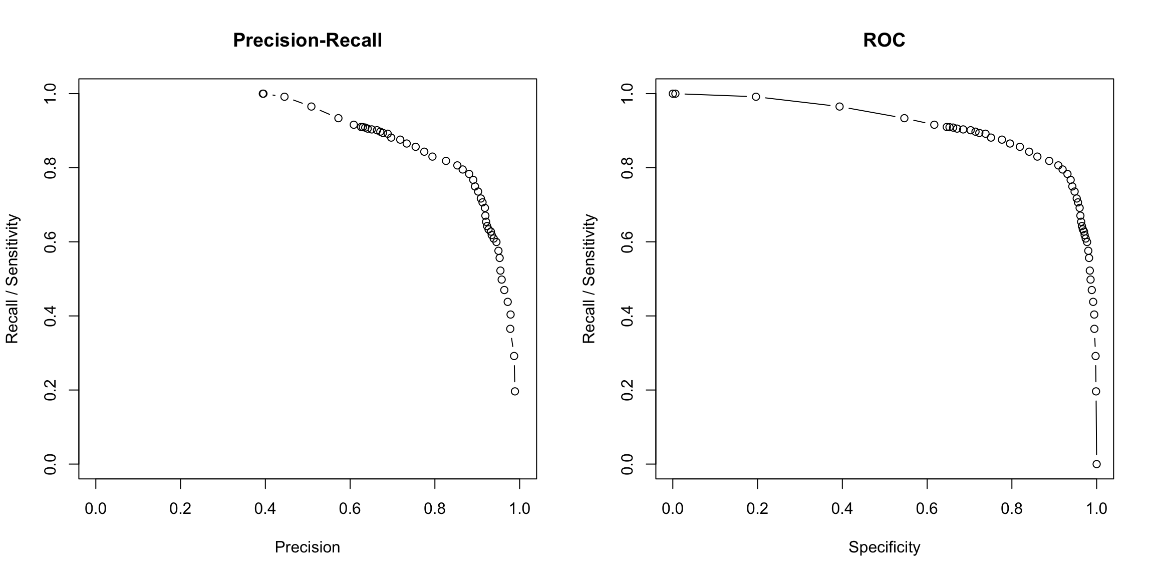
Why would there be a NaN?
We can compare linear and logistic regressions in one plot as follows.
spamlm.precision <- lm.conf[, "C1"]/(lm.conf[, "C1"] +
    glm.conf[, "W1"])
spamlm.recall <- lm.conf[, "C1"]/(lm.conf[, "C1"] +
    glm.conf[, "W0"])
spamlm.spec <- lm.conf[, "C0"]/(lm.conf[, "C0"] + glm.conf[,
    "W1"])
par(mfrow = c(1, 2))
matplot(x = cbind(spamGlm.precision, spamlm.precision),
    y = cbind(spamGlm.recall, spamlm.recall), xlab = "Precision",
    ylab = "Recall", type = "l")
legend(0.8, 0.4, lty = 1:2, col = 1:2, c("glm", "lm"))
matplot(x = cbind(spamGlm.spec, spamlm.spec), y = cbind(spamGlm.recall,
    spamlm.recall), ylab = "Recall / Sensitivity",
    xlab = "Specificity", type = "l")
legend(0.8, 0.4, lty = 1:2, col = 1:2, c("glm", "lm"))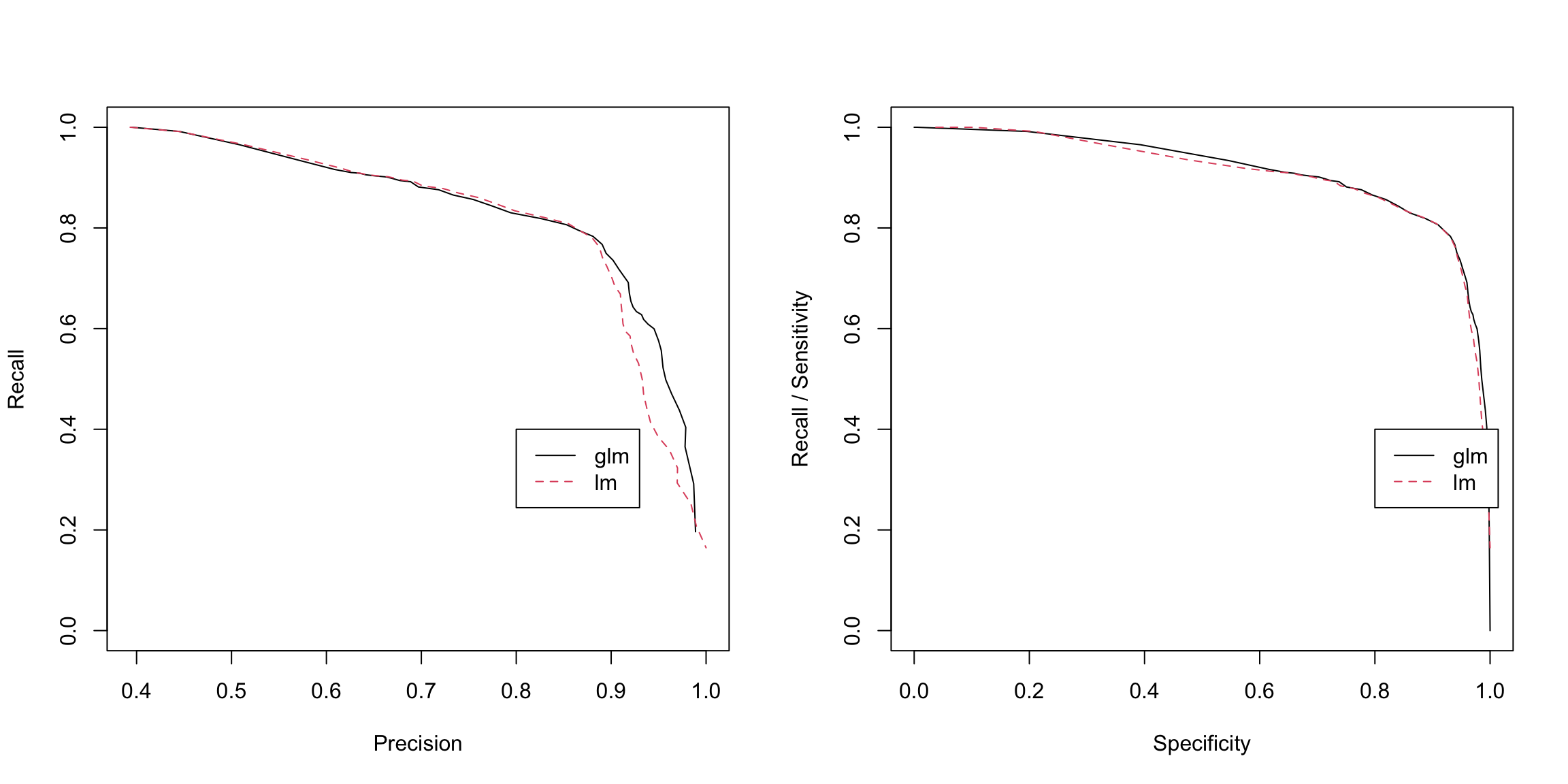
Why one versus the other?
Notice that Precision-Recall focuses on the cases of \(y=1\) or \(\hat{y}=1\). This can be useful in cases where your focus is really on how well you detect someone and you are not concerned about how well you are detecting \(y=0\). This is most common if the vast majority of the population has \(y=0\), and you want to detect very rare events when \(y=1\) – these are often problems when you are “trying to find a needle in the haystack”, and only care about your ability to find positive results. For example, suppose you want to consider how well a search engine lists of links are correctly related to the topic requested. You can imagine all websites in the world have a true \(y_i=1\) if it would be correct to be listed and the search engine gives a \(\hat{y}_i=1\) to those websites that they will return. Then precision is asking (on average) what proportion of the search engine’s list of websites are correct; recall/sensitivity is asking what proportion of all of the \(y_i=1\) websites are found. Both are reasonable questions to try to trade off. Specificity, however, is what proportion of all the other (billion?) websites that are not related (i.e. \(y_i=0)\) are NOT given in the search engine’s list of good websites. You are not concerned about this quantity at all.
However, in other contexts it matters very much how good you are at separating the negative results (i.e. \(y=0\)). Consider predicting if a patient has a disease \((\hat{y}_i=1)\), and then \(y_i\) is whether the patient actually has a disease. A negative result tells a patient that the patient doesn’t have the disease – and is a serious problem if in fact the patient does have the disease, and thus doesn’t get treatment.
Note that the key distinction between these two contexts the reprecussions to being negative. There are many settings where the use of the predictions is ultimately as a recommendation system (movies to see, products to buy, best times to buy something, potential important genes to investigate, etc), so mislabeling some positive things as negative (i.e. not finding them) isn’t a big deal so long as what you do recommend is high quality.
Indeed, the cases where trade-offs lead to different conclusions tend to be cases where the overall proportion of \(y_i=1\) in the population is small. (However, just because they have a small proportion in the population doesn’t mean you don’t care about making mistakes about negatives – missing a diagnosis for a rare but serious disease is still a problem)
I.e. conditional on \(x\), \(y\) is distributed \(Bernoulli(p(x))\).↩
This comes from assuming that the \(y_i\) follow a Bernoulli distribtion with probability \(p_i\). Then this is the negative log-likelihood of the observation, and by minimizing the average of this over all observations, we are maximizing the likelihood.↩
The glm summary gives the Wald-statistics, while the anova uses the likelihood ratio statistic.↩